CHAPTER 12
FEEDBACK LINEARIZATION

In this chapter we present some basic, but fundamental, ideas from geometric nonlinear control theory. We first give some background from differential geometry to set the notation and define basic quantities, such as manifold, vector field, Lie bracket, and so forth that we will need later. The main tool that we will use in this chapter is the Frobenius theorem, which we introduce in Section 12.1.2.

We then discuss the notion of feedback linearization of nonlinear systems. This approach generalizes the concept of inverse dynamics of rigid manipulators discussed in Chapter 9. The idea of feedback linearization is to construct a nonlinear control law as an inner-loop control, which, in the ideal case, exactly linearizes the nonlinear system after a suitable state space change of coordinates. The designer can then design the outer-loop control in the new coordinates to satisfy the traditional control design specifications such as tracking and disturbance rejection.

In the case of rigid manipulators the inverse dynamics control of Chapter 9 and the feedback linearizing control are the same. The main difference between inverse dynamics control and feedback linearization, as we shall see, is to find the “right” set of coordinates with respect to which the dynamics can be rendered linear by feedback. In the case of inverse dynamics, no change of coordinates is necessary.

As we shall see, the full power of the feedback linearization technique for manipulator control becomes apparent if one includes in the dynamic description of the manipulator the transmission dynamics, such as elasticity resulting from shaft windup and gear elasticity.

12.1 Background

In recent years an impressive volume of literature has emerged in the area of differential geometric methods for nonlinear systems, treating not only feedback linearization but also other problems such as disturbance decoupling, estimation, observers, and adaptive control. It is our intent here to give only that portion of the theory that finds an immediate application to robot control, and even then to give only the simplest versions of the results.

12.1.1 Manifolds, Vector Fields, and Distributions

The fundamental notion in differential geometry is that of a differentiable manifold, (manifold for short) which is a topological space that is locally diffeomorphic¹ to Euclidean space . For our purposes here a manifold may be thought of as a subset of defined by the zero set of a smooth vector valued function² , for p < n,

We assume that the differentials dh₁, …, dh_p are linearly independent at each point, in which case the dimension of the manifold is m = n − p. Given an m-dimensional manifold M we may attach at each point x ∈ M a tangent space T_xM, which is an m-dimensional vector space specifying the set of possible velocities (directional derivatives) at x.

Example 12.1.

Consider the unit sphere S² in defined by

S² is a two-dimensional submanifold of .

At points in the upper hemisphere, , and the tangent space is spanned by the vectors

**Figure 12.1** The sphere as a two-dimensional manifold in .

The diagram shows a vector on a manifold. — **Figure 12.2** Pictorial representation of a vector field on a manifold.

The differential of h is

which is perpendicular to the tangent plane at x, y, z.

Definition 12.1.

A smooth vector field on a manifold M is an infinitely differentiable function f: M → TM represented as a column vector

Another useful notion is that of cotangent space and covector field. The cotangent space T*_xM is the dual space of the tangent space. It is an m-dimensional vector space specifying the set of possible differentials of functions at x. Mathematically, T*_xM is the space of all linear functionals on T_xM, that is, the space of functions from T_xM to .

Definition 12.2.

A smooth covector field is a function w: M → T*M, which is infinitely differentiable, represented as a row vector,

Henceforth, whenever we use the term function, vector field, or covector field, it is assumed to be smooth. Since T_xM and T*_xM are m-dimensional vector spaces, they are isomorphic and the only distinction we will make between vectors and covectors below is whether or not they are represented as column vectors or row vectors.

We may also have multiple vector fields defined simultaneously on a given manifold. Such a set of vector fields will span a subspace of the tangent space at each point. Likewise, we will consider multiple covector fields spanning a subspace of the cotangent space at each point. These notions give rise to so-called distributions and codistributions.

Definition 12.3.

Let X₁(x), …, X_k(x) be vector fields on M. A distribution Δ is the linear span of the vectors (at each x ∈ M)

(12.1)

Likewise, let w₁(x), …, w_k(x) be covector fields on M. A codistribution Ω is the linear span of the covectors (at each x ∈ M)

(12.2)

Remark 12.1.

We will assume that the distribution Δ is linearly independent at each x ∈ M, in which case Δ is called a regular distribution. Henceforth, whenever we say distribution, it will be understood to mean regular distribution. The same convention will apply to codistribution and regular codistribution.

A distribution therefore assigns a vector space Δ(x) to each point x ∈ M. Δ(x) is a k-dimensional subspace of the m-dimensional tangent space T_xM. A codistribution likewise defines a k-dimensional subspace Ω(x) at each x of the m-dimensional cotangent space T*_xM.

Vector fields are used to define differential equations and their associated flows. We restrict our attention here to nonlinear systems of the form

(12.3)

where f(x), g₁(x), …, g_m(x) are smooth vector fields on M, and where we define G(x) = [g₁(x), …, g_m(x)] and u = [u₁, …, u_m]^T. In the remainder of this chapter we will assume that .

Definition 12.4.

Let f and g be two vector fields on . The Lie bracket of f and g, denoted by [f, g], is a vector field defined by

(12.4)

where (respectively, ) denotes the n × n Jacobian matrix whose ij^th entry is (respectively, ).

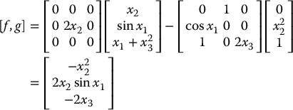
Example 12.2

Suppose that vector fields f(x) and g(x) on are given as

Then the vector field [f, g] is computed according to Equation (12.4) as

We also denote [f, g] as ad_f(g) and define ad^k_f(g) inductively by

(12.5)

with ad⁰_f(g) = g.

Definition 12.5.

Let be a vector field on and let be a scalar function. The Lie derivative of h with respect to f, denoted L_fh, is defined as

(12.6)

The Lie derivative is simply the directional derivative of h in the direction of f. We denote by L²_fh the Lie derivative of L_fh with respect to f, that is,

(12.7)

In general we define

(12.8)

with L⁰_fh = h.

The following technical lemma gives an important relationship between the Lie bracket and Lie derivative and is crucial to the subsequent development.

Lemma 12.1

Let be a scalar function and f and g be vector fields on . Then we have the following identity

(12.9)

Proof:

Expand Equation (12.9) in terms of the coordinates x₁, …, x_n and equate both sides. The i^th component [f, g]_i of the vector field [f, g] is given as

Therefore, the left-hand side of Equation (12.9) is

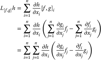
If the right-hand side of Equation (12.9) is expanded similarly it can be shown, with a little algebraic manipulation, that the two sides are equal. The details are left as an exercise (Problem 12–1).

12.1.2 The Frobenius Theorem

In this section we present a basic result in differential geometry known as the Frobenius theorem. The Frobenius theorem can be thought of as an existence theorem for solutions to certain systems of first-order partial differential equations. Although a rigorous proof of this theorem is beyond the scope of this text, we can gain an intuitive understanding of it by considering the following system of partial differential equations

(12.10)

(12.11)

In this example there are two partial differential equations in a single dependent variable z. A solution to Equations (12.10) and (12.11) is a function z = ϕ(x, y) satisfying

(12.12)

(12.13)

We can think of the function z = ϕ(x, y) as defining a surface in as in Figure 12.3. The function defined by

The diagram shows an example of an integral manifold. — **Figure 12.3** Integral manifold in .

(12.14)

then characterizes both the surface and the solution of Equations (12.10) and (12.11). At each point (x, y) the tangent plane to the surface is spanned by two vectors found by taking partial derivatives of Φ in the x and y directions, respectively, that is, by

(12.15)

The vector fields X₁ and X₂ are linearly independent and span a two-dimensional subspace at each point. Notice that X₁ and X₂ are completely specified by Equations (12.10) and (12.11). Geometrically, one can now think of the problem of solving this system of first-order partial differential equations as the problem of finding a surface in whose tangent space at each point is spanned by the vector fields X₁ and X₂. Such a surface, if it can be found, is called an integral manifold for Equations (12.10) and (12.11). If such an integral manifold exists then the set of vector fields, equivalently, the system of partial differential equations, is called completely integrable.

Let us reformulate this problem in yet another way. Suppose that z = ϕ(x, y) is a solution of Equations (12.10) and (12.11). Then it is a simple computation (Problem 12–2) to check that the function

(12.16)

satisfies the system of partial differential equations

(12.17)

Conversely, suppose a scalar function h can be found satisfying (12.17), and suppose that we can solve the equation

(12.18)

for z, as z = ϕ(x, y).³ Then it can be shown (Problem 12–3) that ϕ satisfies Equations (12.10) and (12.11). Hence, complete integrability of the set of vector fields {X₁, X₂} is equivalent to the existence of h satisfying Equations (12.17). With the preceding discussion as background we state the following.

Definition 12.6.

A distribution Δ = span{X₁, …, X_m} on is said to be completely integrable if and only if there are n − m linearly independent functions h₁, …, h_{n − m} satisfying the system of partial differential equations

(12.19)

Another important concept is the notion of involutivity, as defined next.

Definition 12.7.

A distribution Δ = span{X₁, …, X_m} is said to be involutive if and only if there are scalar functions such that

(12.20)

Involutivity simply means that if one forms the Lie bracket of any pair of vector fields in Δ then the resulting vector field can be expressed as a linear combination of the original vector fields X₁, …, X_m. An involutive distribution is thus closed under the operation of taking Lie brackets. Note that the coefficients in this linear combination are allowed to be smooth functions on .

In the simple case of Equations (12.10) and (12.11) one can show that involutivity of the set {X₁, X₂} defined by Equation (12.19) is equivalent to interchangeability of the order of partial derivatives of h, that is, . The Frobenius theorem, stated next, gives the conditions for the existence of a solution to the system of partial differential equations (12.19).

Theroem 12.1. (Frobenius).

A distribution Δ is completely integrable if and only if it is involutive.

The importance of the Frobenius theorem is that it allows one to determine whether or not a given distribution is integrable without having to actually solve the partial differential equations. The involutivity condition can, in principle, be computed from the given vector fields alone.

12.2 Feedback Linearization

To introduce the idea of feedback linearization consider the following simple system,

(12.21)

(12.22)

Note that we cannot simply choose u in the above system to cancel the nonlinear term asin (x₂). However, if we first change variables by setting

(12.23)

(12.24)

then, by the chain rule, y₁ and y₂ satisfy

(12.25)

We see that the nonlinearities can now be cancelled by the control input

(12.26)

which results in the linear system in the (y₁, y₂) coordinates

(12.27)

The term v has the interpretation of an outer-loop control and can be designed to place the poles of the second-order linear system given by Equation (12.27) in the coordinates (y₁, y₂). For example, the outer-loop control

(12.28)

applied to Equation (12.27) results in the closed-loop system

(12.29)

which has characteristic polynomial

(12.30)

and hence, the closed-loop poles of the system with respect to the coordinates (y₁, y₂) are completely specified by the choice of k₁ and k₂. Figure 12.4 illustrates the inner-loop/outer-loop implementation of the above control strategy. The response in the y variables is easy to determine. The corresponding response of the system in the original coordinates (x₁, x₂) can be found by inverting the transformation given by Equations (12.23) and (12.24). The result is

The diagram shows the inner-loop/outer-loop control architecture for feedback linearization. — **Figure 12.4** Inner-loop/outer-loop control architecture for feedback linearization.

(12.31)

This example illustrates several important features of feedback linearization. The first thing to note is the local nature of the result. We see from Equations (12.23) and (12.24) that the transformation and the control make sense only in the region − ∞ < x₁ < ∞, . Second, in order to control the linear system given by Equation (12.27), the coordinates (y₁, y₂) must be available for feedback. This can be accomplished by measuring them directly if they are physically meaningful variables, or by computing them from the measured (x₁, x₂) coordinates using the transformation given by Equations (12.23) and (12.24). In the latter case the parameter a must be known precisely.

In Section 12.3 we give necessary and sufficient conditions under which a general single-input nonlinear system can be transformed into a linear system using a nonlinear change of variables and nonlinear feedback as in the above example.

12.3 Single-Input Systems

The idea of feedback linearization is easiest to understand in the context of single-input systems. In this section we give necessary and sufficient conditions for single-input nonlinear system to be locally feedback linearizable. As an illustration, we apply this result to the control of a single-link manipulator with joint elasticity.

Definition 12.8.

A single-input nonlinear system

(12.32)

where f(x) and g(x) are vector fields on , f(0) = 0, and , is said to be feedback linearizable if there exists a diffeomorphism , defined on an open region U in containing the origin, and nonlinear feedback

(12.33)

with β(x) ≠ 0 on U such that the transformed state

(12.34)

satisfies the linear system of equations

(12.35)

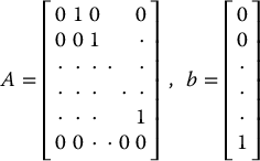
where

(12.36)

Remark 12.2

The linear system (12.35) with A and b given by (12.36) is known as the Brunovsky canonical form. Any controllable single-input linear system can be transformed into the Brunovsky form with a linear change of coordinates and linear state feedback. Thus, it is without loss of generalization that we specify the Brunovsky form as the target linear system in the definition of nonlinear feedback linearization.

The nonlinear transformation given by Equation (12.34) and the nonlinear control law, Equation (12.33), when applied to the nonlinear system (12.32), result in a linear controllable system (12.35). The diffeomorphism T(x) can be thought of as a nonlinear change of coordinates in the state space. The idea of feedback linearization is that, if one first changes to the coordinate system y = T(x), then there exists a nonlinear control law to cancel the nonlinearities in the system. The feedback linearization is said to be global if the region U is all of .

We next derive necessary and sufficient conditions on the vector fields f and g in Equation (12.32) for the existence of such a nonlinear coordinate transformation. Let us set

(12.37)

and see what conditions the transformation T(x) must satisfy. Differentiating both sides of Equation (12.37) with respect to time yields

(12.38)

where is the Jacobian matrix of the transformation T(x). Using Equations (12.32) and (12.35), Equation (12.38) can be written as

(12.39)

In component form with

(12.40)

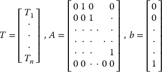
we see that the first equation in Equation (12.39) is

(12.41)

Similarly, the other components of T satisfy

(12.42)

Since we assume that T₁, …, T_n are independent of u while v is not independent of u we conclude from (12.42) that

(12.43)

(12.44)

This leads to the system of partial differential equations

(12.45)

together with

(12.46)

Using Lemma 12.1 together with Equations (12.43) and (12.44) we can derive a system of partial differential equations in terms of T₁ alone as follows. Using h = T₁ in Lemma 12.1 we have

(12.47)

Thus, we have shown

(12.48)

By proceeding inductively it can be shown (Problem 12–4) that

(12.49)

(12.50)

If we can find T₁ satisfying the system of partial differential equations (12.49), then T₂, …, T_n are found inductively from Equation (12.45) and the control input u is found from (12.46) as

(12.51)

We have thus reduced the problem to solving the system given by Equation (12.49) for T₁. When does such a solution exist?

First note that the vector fields g, ad_f(g), …, ad^{n − 1}_f(g) must be linearly independent. If they are not linearly independent, then for some index i, we would have

(12.52)

and then ad^{n − 1}_f(g) would be a linear combination of g, ad_f(g), …, ad^{n − 2}_f(g) and Equation (12.50) could not hold. Now, by the Frobenius theorem, Equation (12.49) has a solution if and only if the distribution Δ = span{g, ad_f(g), …, ad^{n − 2}_f(g)} is involutive. Putting this together we have shown the following

Theroem 12.2.

The nonlinear system

(12.53)

is feedback linearizable if and only if there exists an open region U containing the origin in in which the following conditions hold:

The vector fields {g, ad_f(g), …, ad^{n − 1}_f(g)} are linearly independent in U.
The distribution Δ = span{g, ad_f(g), …, ad^{n − 2}_f(g)} is involutive in U.

Remark 12.3.

A few remarks about the above theorem are the following:

For a linear system,
it is easily shown that ad^k_f(g) = −1^kF^kg (Problem 12–5) and therefore the first condition above is equivalent to controllability of the pair F, g.
Since each term ad^k_f(g) is constant, the involutivity condition is trivially satisfied, since the Lie bracket of two constant vector fields is zero. Therefore, controllability in the linear case is necessary and sufficient to transform the system into the Brunovsky canonical form with a linear change of variables and linear state feedback.
A necessary condition for the nonlinear system
to be feedback linearizable is that the linear approximation about the origin
is controllable.
For second-order systems, controllability of the linear approximation about the origin is both necessary and sufficient for feedback linearizability. This follows immediately from the fact that the distribution Δ in the case n = 2 is Δ = span{g(x)} since a one-dimensional distribution is always involutive.

Example 12.3. (Flexible-Joint Robot).

Consider the single-link, flexible-joint manipulator shown in Figure 12.5. Ignoring damping for simplicity, the equations of motion are

(12.54)

Note that since the nonlinearity enters into the first equation the control u cannot simply be chosen to cancel it as in the case of the rigid manipulator equations. In state space we set

(12.55)

and write the system (12.54) as

(12.56)

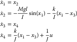
The system is thus of the form (12.32) with

(12.57)

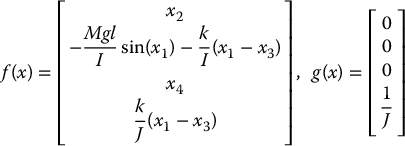
Therefore, with n = 4, the necessary and sufficient conditions for feedback linearization of this system are that

(12.58)

and that the distribution

(12.59)

is involutive. Performing the indicated calculations it is easy to check that (Problem 12–10)

(12.60)

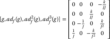
which has rank 4 for k, I, J ≠ 0. Also, since the vector fields {g, ad_f(g), ad²_f(g)} are constant, the distribution Δ is involutive. To see this it suffices to note that the Lie bracket of two constant vector fields is zero. Hence, the Lie bracket of any two members of the set of vector fields in Equation (12.59) is zero, which is trivially a linear combination of the vector fields themselves. It follows that the system given by Equation (12.54) is feedback linearizable. The new coordinates

(12.61)

are found from the conditions given by Equation (12.49), with n = 4, that is

(12.62)

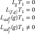
Carrying out the above calculations leads to the system of equations (Problem 12–11)

(12.63)

and

(12.64)

From this we see that the function T₁ should be a function of x₁ alone. Therefore, we take the simplest solution

(12.65)

and compute from Equation (12.45) (Problem 12–12)

(12.66)

The feedback linearizing control input u is found from the condition

(12.67)

as (Problem 12–13)

(12.68)

where

(12.69)

Therefore in the coordinates y₁, …, y₄ with the control law given by Equation (12.68) the system becomes

(12.70)

or, in matrix form,

(12.71)

where

(12.72)

It is interesting to note that the above feedback linearization is actually global. In order to see this we need only compute the inverse of the change of variables given by Equations (12.65) and (12.66). By inspection we see that

(12.73)

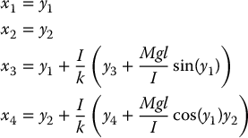
The inverse transformation is well defined and differentiable everywhere and, hence, the feedback linearization for the system given by Equation (12.54) holds globally. The transformed variables y₁, …, y₄ are themselves physically meaningful. We see that

(12.74)

Since the motion trajectory of the link is typically specified in terms of these quantities, they are natural variables to use for feedback.

Example 12.4.

Once the system is linearized to Brunovsky form, we can choose the outer-loop control v as

to execute a step change y^ref₁ in the link angle.

Figure 12.6 shows the response of the system with parameter values I = J = 1, mgL = 10, k = 100, reference value y^ref₁ = π/2, and outer loop gains k₁ = 4788, k₂ = 2319, k₃ = 420, k₄ = 34, chosen so that the closed poles of the linearized system are at − 7, −8, −9, −9.5. Note that the final value of the input torque is u = 10, which is necessary to balance the gravitational torque mgL = 10.

The figure shows the single-link, flexible joint robot. — **Figure 12.5** Single-link, flexible joint robot.

Illustration shows two graphs.
(a) A graph is shown in the xy-plane. The x-axis represents “time (sec)” ranges from 0 to 2. The y-axis represents “angle (rad)” ranges from 0 to 2. The graph shows the step response of the flexible joint robot.
(b) A graph is shown in the xy-plane. The x-axis represents “time (sec)” ranges from 0 to 2. The y-axis represents “torque (Nm)” ranges from negative 20 to positive 80. The graph shows the motor torque of the flexible joint robot. — **Figure 12.6** Step response and motor torque of the flexible joint robot. The difference between the final values of the motor angle and the link angle are determined by the joint stiffness and the steady-state value of the gravitational torque.

Example 12.5.

The next example shows the response for the above flexible joint robot, where the reference input is a cubic polynomial trajectory. With a cubic polynomial the desired jerk is a constant. Therefore, let us specify a trajectory

(12.75)

so that

Then a linear control law that tracks this trajectory, which is essentially equivalent to the feedforward/feedback scheme of Chapter 9, is given by

(12.76)

Applying this control law to the fourth-order linear system given by Equation (12.68) we see that the tracking error e(t) = y₁ − y^d₁ satisfies the fourth-order linear equation

(12.77)

and, hence, the error dynamics are completely determined by the choice of gains k₀, …, k₃.

Figure 12.7 shows the closed loop response of the system.

Remark 12.4.

Notice that the feedback control law given by Equation (12.76) is stated in terms of the variables y₁, …, y₄. Thus, it is important to consider how these variables are to be determined so that they may be used for feedback in case they cannot be measured directly. Although the first two variables, representing the link position and velocity, are easy to measure, the remaining variables, representing link acceleration and jerk, are difficult to measure with any degree of accuracy using present technology. One could measure the original variables x₁, …, x₄, which represent the motor and link positions and velocities, and compute y₁, …, y₄ using the transformation Equations (12.65) and (12.66). In this case the parameters appearing in the transformation equations would have to be known precisely. One may also implement a nonlinear observer to estimate the full state, given only the measured link position x₁.

Nonlinear Observer with Output Injection

It is interesting to note that the special structure of the dynamic equations (12.54), in the single-link case, allows us to design a nonlinear observer to estimate the full state vector, x = [x₁, x₂, x₃, x₄]^T supposing that only the link angle x₁ is measured. To see this, set y = x₁ = c^Tx as an output equation with c^T = [1, 0, 0, 0]. We can then write the state space equations (12.56) as

where

(12.78)

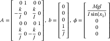
Since ϕ(y) is a nonlinear function depending only on the output y, a so-called nonlinear observer with output injection takes the form

The estimation error is then given by the linear system

(12.79)

It is easily checked that (c^T, A) is an observable pair and so the observer gains ℓ can now be chosen so that A − ℓc^T is a Hurwitz matrix. Figure 12.8 shows the closed-loop response of the system using the estimated state in the control input. The observer gains were chosen as ℓ₁ = 46, ℓ₂ = 591, ℓ₃ = 14.3, ℓ₄ = −419.

12.4 Multi-Input Systems

In the general case of an n-link manipulator the dynamic equations represent a multi-input nonlinear system. The conditions for feedback linearization of multi-input systems are more difficult to state, but the conceptual idea is the same as the single-input case. That is, one seeks a coordinate system in which the nonlinearities can be exactly cancelled by one or more of the inputs. In the multi-input system we can also decouple the system, that is, linearize the system in such a way that the resulting linear system is composed of subsystems, each of which is affected by only a single one of the outer-loop control inputs.

Since we are concerned only with the application of these ideas to manipulator control, we will not need the most general results in multi-input feedback linearization. Instead, we will use the physical insight gained by our detailed derivation of this result in the single-link case to derive a feedback linearizing control both for n-link rigid manipulators and for n-link manipulators with elastic joints. For fully-actuated rigid manipulators, no coordinate change from the usual generalized coordinates is needed. For n-link flexible-joint robots, the required coordinate transformation can be defined in terms of the link position, velocity, acceleration, and jerk just as in the single-input case.

Example 12.6.

We will first verify what we have stated previously, namely that for an n-link rigid manipulator the feedback linearizing control is identical to the inverse dynamics control of Chapter 9. To see this, consider the rigid robot equations of motion given by Equation (9.2.6), which we write in state space as

(12.80)

with x₁ = q, . In this case a feedback linearizing control is found by simply inspecting Equation (12.80) as

(12.81)

Substituting Equation (12.81) into Equation (12.80) yields

(12.82)

Equation (12.82) represents a set of n second-order systems of the form

(12.83)

Comparing Equation (12.81) with Equation (9.3.4) we see indeed that the feedback linearizing control for a rigid manipulator is precisely the inverse dynamics control of Chapter 9.

Example 12.7

Including the joint flexibility in the dynamic description of an n-link robot results in a Lagrangian system with 2n degrees of freedom. Recall the Euler–Lagrange equations of motion for the flexible-joint robot from Chapter 9

(12.84)

In state space, which is now , we define state variables in block form

(12.85)

Then from Equation (12.84) we have:

(12.86)

where we define h(x₁, x₂) = C(x₁, x₂)x₂ + g(x₁) for simplicity. This system is of the form

(12.87)

In the single-link case we saw that the system could be linearized by nonlinear feedback if we took as state variables the link position, velocity, acceleration, and jerk. Following the single-input example, we can attempt to do the same thing in the multi-link case and derive a feedback linearizing transformation blockwise as follows. Set

(12.88)

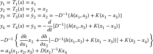
where for simplicity we define the function a₄ to be everything in the definition of y₄ except the last term, which is D^{− 1}Kx₄. Note that x₄ appears only in this last term so that a₄ depends only on x₁, x₂, x₃.

As in the single-link case, the above mapping is a global diffeomorphism. Its inverse can be found by inspection to be

(12.89)

The linearizing control law can now be found from the condition

(12.90)

Computing from Equation (12.88) yields

(12.91)

where a(x) denotes all the terms in Equation (12.91) but the last term, which involves the input u, and b(x) = D^{− 1}(x)KJ^{− 1}.

Solving the above expression for u yields

(12.92)

where β(x) = JK^{− 1}D(x) and α(x) = −b(x)^{− 1}a(x).

With the nonlinear change of coordinates given by Equation (12.88) and nonlinear feedback given by Equation (12.92) the transformed system now has the linear block form

(12.93)

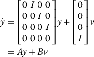
where I = n × n identity matrix, 0 = n × n zero matrix, , and . The system (12.93) represents a set of n decoupled quadruple integrators. The outer-loop design can now proceed as before, because not only is the system linearized, but it consists of n subsystems each identical to the fourth-order system (12.70).

12.5 Chapter Summary

This chapter introduced some basic concepts from differential geometric nonlinear control theory and serves as a foundation to explore more advanced literature.

Manifolds, Vector Fields, Distributions

We introduced basic definitions from differential geometry, such as a differentiable manifold, vector field, and distribution. We introduced some geometric operations such as the Lie derivative and Lie bracket and showed how they are related. We stated the Frobenius Theorem, which is an important tool for nonlinear analysis.

Feedback Linearization

We derived the necessary and sufficient conditions for feedback linearization of single-input nonlinear systems. This important result serves as a basis for controller design for a wide range of physical systems. In particular, we showed how feedback linearization can be used to design globally stable tracking controllers for flexible joint robots.

Problems

Complete the proof of Lemma 12.1 by direct calculation.
Show that the function h = z − ϕ(x, y) satisfies the system given by Equation (12.17) if ϕ is a solution of Equations (12.10) and (12.11) and X₁, X₂ are defined by Equation (12.15).
Show that if h(x, y, z) satisfies Equation (12.17) and , then Equation (12.18) can be solved for z as z = ϕ(x, y) where ϕ satisfies Equations (12.10) and (12.11). Also show that can occur only in the case of the trivial solution h = 0 of Equation (12.17).
Verify Equations (12.49) and (12.50).
Show that if F and g are n × n and n × 1, respectively, that
Is the second-order system below feedback linearizable about the origin? Prove your answer.
Show that the system below is locally feedback linearizable.
Find explicitly the change of coordinates and nonlinear feedback to linearize the system.
Derive Equation (12.54), which gives the equations of motion for the single-link manipulator with joint elasticity of Figure 12.5 using Lagrange’s equations.
Repeat Problem 12–8 if there is viscous friction both on the link side and on the motor side of the spring in Figure 12.5.
Perform the calculations necessary to verify Equation (12.60).
Derive the system of partial differential equations (12.63) from the condition (12.62). Also verify Equation (12.64).
Compute the change of coordinates (12.66).
Verify Equations (12.68) and (12.69).
Verify Equations (12.73).
Design and simulate a linear outer-loop control law v for the system given by Equation (12.54) so that the link angle y₁(t) follows a desired trajectory y^d₁(t) = θ_ℓ^d(t) = sin 8t. Use various techniques such as pole placement, linear quadratic optimal control, etc.
Consider again a single-link manipulator (either rigid or elastic joint). Add to your equations of motion the dynamics of a permanent magnet DC motor. What can you say now about feedback linearizability of the system?
What happens to the inverse coordinate transformation given by Equation (12.73) as the joint stiffness k → ∞? Give a physical interpretation. Use this to show that the system given by Equation (12.54) reduces to the equation governing the rigid joint manipulator in the limit as k → ∞.
Consider the single-link manipulator with elastic joint of Figure 12.5 but suppose that the spring characteristic is nonlinear, that is, suppose that the spring force F is given by F = ϕ(q₁ − q₂), where ϕ is a diffeomorphism. Derive conditions under which the system is feedback linearizable and carry out the details of the feedback linearizing transformation. Specialize the result to the case of a cubic spring characteristic ϕ = k₁(q₁ − q₂) + (q₁ − q₂)³. The cubic spring characteristic is a more accurate description for many manipulators than is the linear spring, especially for elasticity arising from gear flexibility.

Notes and References

A rigorous treatment of differential geometry can be found, for example, in a number of texts, for example, [15] or [156]. A comprehensive treatment of differential geometric methods in control is [69]. For specific applications in robotics of these advanced methods, the reader is referred to [118] and [32].

Our treatment of feedback linearization for single-input, affine, nonlinear systems follows closely the pioneering result of Su [171]. The first application of the method of feedback linearization for the single-link flexible-joint robot appeared in Marino and Spong [109]. The corresponding result for the case of n-link flexible-joint robots is due to Spong [165]. Dynamic feedback linearization for flexible-joint robots was treated in DeLuca [34]. An complete reference for flexible-joint robots is in Readman [142]. The problem of designing nonlinear observers is treated in [81] and [82].

Notes

¹ A diffeomorphism is simply a differentiable function whose inverse exists and is also differentiable. We shall assume both the function and its inverse to be infinitely differentiable. Such functions are customarily referred to as C^∞ diffeomorphisms.
² Our definition amounts to the special case of an embedded submanifold of dimension m = n − p in .
³ The implicit function theorem states that Equation (12.18) can be solved for z as long as .

ϕ ϕ