CHAPTER 9
NONLINEAR AND MULTIVARIABLE CONTROL
9.1 Introduction
In Chapter 8 we discussed techniques to derive control laws for each joint of a manipulator based on a single-input/single-output model. Coupling effects among the joints were regarded as disturbances to the individual systems. In reality, the dynamic equations of a robot manipulator form a complex, nonlinear, and multivariable system. In this chapter, therefore, we treat the robot control problem in the context of nonlinear, multivariable control. This approach allows us to provide more rigorous analysis of the performance of control systems, and also allows us to design robust and adaptive nonlinear control laws that guarantee stability and tracking of planned trajectories.
We first reformulate the manipulator dynamic equations in a form more suitable for the discussion to follow. We then treat the problem of inverse dynamics in both joint space and task space. The inverse dynamics control relies on exact cancellation of nonlinearities in the system, which is not possible in practical applications. For this reason, we discuss several methods for robust and adaptive control, which are aimed at providing good tracking performance despite uncertainty in knowledge of parameters or external disturbances. In distinguishing between robust control and adaptive control we follow the commonly accepted notion that a robust controller is a fixed controller designed to satisfy performance specifications over a given range of uncertainties, whereas an adaptive controller incorporates some sort of online parameter estimation. This distinction is important. For example, in a repetitive motion task, the tracking errors produced by a fixed robust controller would tend to be repetitive as well, whereas tracking errors produced by an adaptive controller might be expected to decrease over time as the plant and/or control parameters are updated based on runtime information. At the same time, adaptive controllers that perform well in the face of parametric uncertainty may not perform well in the face of other types of uncertainty such as external disturbances or unmodeled dynamics. Therefore, an understanding of the trade-offs involved is important in deciding whether to employ robust or adaptive control design methods in a given situation. The final section outlines a torque optimization procedure to modify any of the controllers in this chapter to account for actuator saturation.
Dynamics Revisited
Recall the robot equations of motion given by Equation (6.65) and the actuator dynamics given by Equation (8.15)
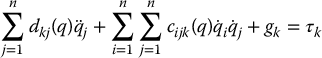

for k = 1, …, n, where  . Multiplying Equation (9.2) by the gear ratio rk and using the fact that the motor angles
  and the link angles qk are related by

we may write Equation (9.2) as

Substituting Equation (9.4) into Equation (9.1) yields
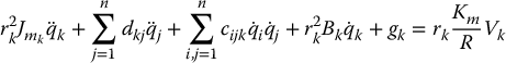
for k = 1, …, n. In matrix form Equation (9.5) can be written as

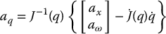
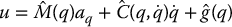
where M(q) = D(q) + J with J a diagonal matrix with diagonal elements r2kJmk. The gravity vector g(q) and the matrix  defining the Coriolis and centrifugal generalized forces are defined as before in Equations (6.67) and (6.68). The input vector u has components

and has units of torque. Note that the above formulation with J assumed to be a diagonal matrix amounts to ignoring the rotation of the motor about axes other than the axis of the joint to which it is attached. However, these off-diagonal effects are typically negligible.
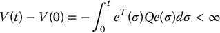
Henceforth, we will ignore the friction and use Equation (9.6) with B = 0 as the plant model for our subsequent development. We leave it as an exercise for the reader (Problem 9–1) to show that the properties of passivity, skew symmetry, bounds on the inertia matrix, and linearity in the parameters continue to hold for the system (9.6).
9.2 PD Control Revisited
It is a rather remarkable fact that the simple PD control scheme that we discussed in Chapter 8 for the set-point control of a single-DOF model can be rigorously shown to work in the general case of Equation (9.6).1 An independent joint PD control scheme can be written in vector form as
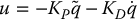
where  is the error between the joint vector q and the desired joint vector qd (the set point), and KP, KD are diagonal matrices of (positive) proportional and derivative gains, respectively. We first show that, in the absence of gravity, that is, if g(q) is zero in Equation (9.6), the PD control law given in Equation (9.7) achieves global asymptotic tracking of the desired joint positions. This, in effect, reproduces the result derived previously but is more rigorous, in the sense that the nonlinear coupling terms are not approximated by a constant disturbance.
To show that the control law given in Equation (9.7) achieves asymptotic tracking consider the Lyapunov function candidate

The first term in Equation (9.8) is the kinetic energy of the robot and the second term accounts for the proportional feedback  . Note that V represents the total energy that would result if the joint actuators were replaced by springs with stiffness constants represented by KP and with equilibrium positions at qd. Thus, V is positive except at the “goal” configuration q = qd,
  , at which point V is zero. The idea is to show that along any motion of the robot, the function V is decreasing to zero. This will imply that the robot is moving toward the desired goal configuration.
To show this we note that, since qd is constant, the time derivative of V is given by

Solving for  in Equation (9.6) with g(q) = 0 and substituting the resulting expression into Equation (9.9) yields
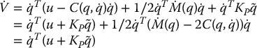
where in the last equality we have used the fact that  is skew symmetric. Substituting the PD control law (9.7) for u into the above yields
The above analysis shows that V is decreasing as long as  is not zero. This by itself is not enough to prove the desired result since it is conceivable that the manipulator could reach a position where
  but q ≠ qd. To show that this cannot happen we can use LaSalle’s theorem (Appendix C). Suppose
  .2 Then Equation (9.11) implies that
  and hence
  . From the equations of motion with PD control

we must then have

which implies that  . LaSalle’s theorem then implies that the equilibrium is globally asymptotically stable.
In case there are gravitational terms present in Equation (9.6), then Equation (9.10) becomes
The presence of the gravitational term in Equation (9.12) means that PD control alone cannot guarantee asymptotic tracking. In practice there will be a steady-state error or offset. Assuming that the closed-loop system is stable and that the joint velocity  goes to zero, the steady-state robot configuration q will satisfy
The physical interpretation of Equation (9.13) is that the configuration q must be such that the motor generates a steady-state “holding torque” KP(q − qd) sufficient to balance the gravitational torque g(q). Thus, we see that the steady-state error can be reduced by increasing the position gain KP.
In order to remove this steady state error we can modify the PD control law as

The modified control law given by Equation (9.14), in effect, cancels the gravitational terms and we achieve the same Equation (9.11) as before. The control law given by Equation (9.14) requires the computation of the gravitational terms g(q) from the Lagrangian equations at each instant of time. If these terms are uncertain, then the control law (9.14) cannot be computed precisely. We will say more about this and related issues later in the context of robust and adaptive control.
The Effect of Joint Flexibility
In Chapter 8 we considered the effect of joint flexibility and showed for a lumped model of a single-link robot that a PD control could be designed for set-point tracking. In this section we will discuss the analogous result in the general case of an n-link manipulator.
We first derive a model similar to Equation (9.6) to represent the dynamics of an n-link robot with joint flexibility. For simplicity, assume that the joints are revolute and are actuated by permanent magnet DC motors. We model the flexibility of the ith joint as a linear torsional spring with stiffness constant ki, for i = 1, …, n.
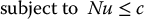
Referring to Figure 9.1, we let q1 = [θ1, ⋅⋅⋅, θn]T be the vector of DH-joint variables and q2 = be the vector of motor shaft angles (reflected to the link side of the gears). Then q1 − q2 is the vector of elastic joint deflections. Neglecting the effect of link motion on the kinetic energy of the actuators, as we did in Equation (9.6), the kinetic and potential energies of the manipulator are given by
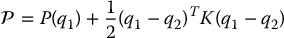
where J and K are diagonal matrices of inertia and stiffness constants, respectively.
Note that we have simply augmented the kinetic energy of the rigid joint robot with the kinetic energy of the actuators and we have likewise augmented the potential energy due to gravity of the rigid joint model with the elastic potential energy of the linear springs at the joints. It is now straightforward to compute the Euler–Lagrange equations for this system as (Problem 9–2)
For the problem of set-point tracking with PD control, consider a control law of the form
where  and qd is a vector of constant set points, and suppose again that the gravity vector g(q1) = 0. To show asymptotic tracking for the closed-loop system consider the Lyapunov function candidate

We leave it as an exercise (Problem 9–3) to show that an application of LaSalle’s theorem proves global asymptotic stability of the system. Consequently, the motor and link angles are equal in the steady state. Thus, one may choose the set point qd2 as a vector of desired DH variables.

Figure 9.1 A single link of a flexible-joint manipulator. The joint elasticity is represented by a torsional spring between the link angle θi and the motor shaft angle θmi.
If gravity is present, then it is not apparent how one can achieve gravity compensation in a manner similar to the rigid joint case. We will address this question later in the context of feedback linearization in Chapter 12.
9.3 Inverse Dynamics
We now consider the application of more complex nonlinear control techniques for trajectory tracking of rigid manipulators. The first algorithm that we consider is known as the method of inverse dynamics. The method of inverse dynamics is, as we shall see in Chapter 12, a special case of the method of feedback linearization.
After presenting the basic idea of inverse dynamics, both in joint space and in task space, we will discuss the practical situation of uncertainty in the parameters defining the manipulator dynamics. The problem of parametric uncertainty naturally leads to a discussion of robust and adaptive control, which we will discuss in the remaining sections of this chapter.
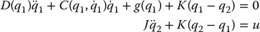
9.3.1 Joint Space Inverse Dynamics
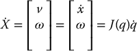
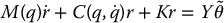
Consider again the dynamic equations of an n-link rigid robot in matrix form

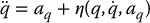
The idea of inverse dynamics is to seek a nonlinear feedback control law

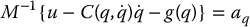
which, when substituted into Equation (9.21), results in a linear closed-loop system. For general nonlinear systems, such a control law may be quite difficult or impossible to find. In the case of the manipulator dynamics given by Equations (9.21), however, the problem is actually easy. By inspecting Equation (9.21) we see that if we choose the control u according to the equation

then, since the inertia matrix M is invertible, the combined system given by Equations (9.21)–(9.23) reduces to

The term aq represents a new input that is yet to be chosen. Equation (9.24) is known as the double integrator system as it represents n uncoupled double integrators. Equation (9.23) is called the inverse dynamics control and achieves a rather remarkable result, namely that the system given by Equation (9.24) is linear and decoupled. This means that each input  can be designed to control a SISO linear system. Moreover, assuming that
  is a function only of qk and
  , then the closed-loop system will be decoupled.
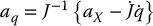
Since aq can now be designed to control a linear second-order system, an obvious choice is to set

where  ,
,  , K0, K1 are diagonal matrices with diagonal elements consisting of position and velocity gains, respectively and the reference trajectory
defines the desired time history of joint positions, velocities, and accelerations. Note that Equation (9.25) is nothing more than a PD control with feedforward acceleration as defined in Chapter 8.
Substituting Equation (9.25) into Equation (9.24), results in
A simple choice for the gain matrices K0 and K1 is
which results in a decoupled closed-loop system with each joint response equal to the response of a critically damped linear second-order system with natural frequency ωi. As before, the natural frequency ωi determines the speed of response of the joint, or equivalently, the rate of decay of the tracking error.
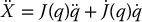
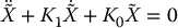
The inverse dynamics approach is important as a basis for control and it is worthwhile to examine it from alternative viewpoints. We can give a second interpretation of the control law (9.23) as follows. Consider again the manipulator dynamics (9.21). Since M(q) is invertible for all  , we may solve for the acceleration
  of the manipulator as

Suppose we were able to specify the acceleration as the input to the system. That is, suppose we had actuators capable of producing directly a commanded acceleration (rather than indirectly by producing a force or torque). Then the dynamics of the manipulator, which is after all a position control device, would be given as

where aq(t) is the input acceleration vector. This is again the familiar double integrator system. Note that Equation (9.30) is not an approximation in any sense; rather it represents the actual open-loop dynamics of the system provided that the acceleration is chosen as the input. The control problem for the system (9.30) is now easy and the acceleration input aq can be chosen as before according to Equation (9.25).
In reality, however, such “acceleration actuators” are not available to us and we must be content with the ability to produce a generalized force (torque) ui at each joint i. Comparing Equations (9.29) and (9.30) we see that the torque input u and the acceleration input aq of the manipulator are related by
Solving Equation (9.31) for the input torque u(t) yields

which is the same as the previously derived expression (9.23). Thus, the inverse dynamics can be viewed as an input transformation that transforms the problem from one of choosing torque input commands to one of choosing acceleration input commands.
Note that the implementation of this control scheme requires the real-time computation of the inertia matrix and the vectors of Coriolis, centrifugal, and gravitational generalized forces. An important issue therefore in the control system implementation is the design of the computer architecture for the above computations.
Figure 9.2 illustrates the so-called inner-loop/outer-loop control architecture. By this we mean that the computation of the nonlinear control law (9.23) is performed in an inner loop with the vectors  , and aq as its inputs and u as output. The outer loop in the system is then the computation of the additional input term aq. Note that the outer-loop control aq is more in line with the notion of a feedback control in the usual sense of being error driven. The design of the outer-loop feedback control is in theory greatly simplified since it is designed for the plant represented by the dotted lines in Figure 9.2, which is now a linear system.

Figure 9.2 Inner-loop/outer-loop control architecture. The inner-loop control computes the vector u of input torques as a function of the measured joint positions and velocities and the given outer-loop control in order to compensate the nonlinearities in the plant model. The outer-loop control designed to track a given reference trajectory can then be based on a linear and decoupled plant model.
9.3.2 Task Space Inverse Dynamics
As an illustration of the importance of the inner-loop/outer-loop control architecture, we will show that tracking in task space can be achieved by modifying the outer-loop control aq in Equation (9.24) while leaving the inner-loop control unchanged. Let  represent the end-effector pose using any minimal representation of SO(3). Since X is a function of the joint variables
  , we have

where J = Ja is the analytical Jacobian of Equation (4.88). Given the double integrator system (9.24) in joint space we see that if aq is chosen as
the result is a double integrator system in task space coordinates

Given a task space trajectory Xd(t) satisfying the same smoothness and boundedness assumptions as the joint space trajectory qd(t), we may choose aX as

so that the task space tracking error  satisfies
Therefore, a modification of the outer-loop control term aq achieves a linear and decoupled system directly in the task space coordinates without the need to compute a joint space trajectory and without the need to modify the nonlinear inner-loop control.
Note that we have used a minimal representation for the orientation of the end effector in order to specify a trajectory  . In general, if the end-effector coordinates are given in SE(3), then the Jacobian J in the above formulation will be the geometric Jacobian of Equation (4.41). In this case
and the outer-loop control
applied to Equation (9.24) results in the system

Although, in this latter case, the dynamics have not been linearized to a double integrator, the outer-loop terms av and aω may still be used to define control laws to track end-effector trajectories in SE(3).
In both cases we see that nonsingularity of the Jacobian is necessary to implement the outer-loop control. Avoiding singularities, therefore, is an important aspect of motion planning and trajectory planning that we have considered in Chapter 7. Also, if the robot has more or fewer than six joints, then the Jacobians are not square. In this case, other schemes have been developed using, for example, the Jacobian pseudoinverse. See [32] for details.
9.3.3 Robust Inverse Dynamics
The inverse dynamics approach relies on exact cancellation of nonlinearities in the robot equations of motion. The practical implementation of inverse dynamics control requires consideration of various sources of uncertainties such as modeling errors, unknown loads, and computation errors. Let us return to the Euler–Lagrange equations of motion

and write the inverse dynamics control input u as
where the notation  represents the computed or nominal value of ( · ) and indicates that the theoretically exact inverse dynamics control is not achievable in practice due to the uncertainties in the system. The error or mismatch
  is a measure of one’s knowledge of the system parameters.
If we substitute Equation (9.45) into Equation (9.44) we obtain, after some algebra (Problem 9–8),
where the nonlinear function  is given by
and is called the uncertainty. Henceforth, we will drop the arguments of  for simplicity. However, it is important to keep in mind that η is, in general, a function of both the state and the reference trajectory.
We define E = E(q) as

which allows us to express the uncertainty η as
The system (9.46) is still nonlinear and coupled due to the uncertainty  and, therefore, we have no guarantee that the outer-loop control given by Equation (9.25) will satisfy desired tracking performance specifications.
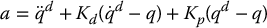
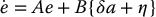
In this section we show how to modify the outer-loop control (9.25) to guarantee global convergence of the tracking error for the system (9.46). The method we outline below is often called Lyapunov redesign. In this approach we set the outer-loop control aq as
where δa is an additional term to be designed. In terms of the tracking error
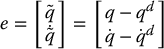
we may write Equations (9.46) and (9.50) as
where
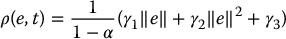
Thus, the double integrator is first stabilized by the linear feedback term  , and the additional control term δa should be designed to overcome the potentially destabilizing effect of the uncertainty η. The basic idea is to assume that we are able to compute a bound ρ(e, t) ⩾ 0 on the uncertainty η as

and design the additional input term δa to guarantee ultimate boundedness of the error trajectory e(t) in Equation (9.52). Note that the bound ρ is in general a function of the tracking error e and time reflecting the fact that η likewise depends on e as well as on t through a time-varying reference trajectory.
Returning to our expression for the uncertainty η and substituting for aq from Equation (9.50) we have
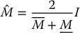
Let us assume that we can find constants α < 1, γ1, and γ2, together with possibly time-varying γ3 such that

We note that the condition  determines how close our estimate
  must be to the true inertia matrix. Suppose that we have constant bounds on M− 1 as

Remark 9.1.
Such constant bounds exist for all robots with revolute joints since the configuration space is compact. The inertia matrices of robots with both revolute and prismatic joints may or may not have constant bounds as in (9.57). See [53] for a complete characterization of manipulator designs satisfying (9.57).
If we choose the estimated inertia matrix  as
as
then it can be shown that
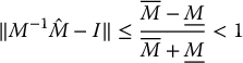
The point is that there is always a choice for  that satisfies the condition ‖E‖ < 1 provided upper and lower bounds
  and
and  can be determined.
Next, assume, for the moment, that ‖δa‖ ⩽ ρ(e, t) which must then be checked a posteriori. It follows that

which, since α < 1, defines ρ as
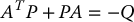
Since K0 and K1 are chosen so that the matrix A in Equation (9.52) is Hurwitz, we may choose Q > 0 and let P > 0 be the unique symmetric positive definite matrix satisfying the Lyapunov equation
Defining the control δa according to
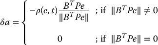
it follows that the Lyapunov function

satisfies  along solution trajectories of Equation (9.52). To show this result, we compute

For simplicity set w = BTPe and consider the second term wT{δa + η} in the above expression. If w = 0 this term vanishes, and hence,
independent of the choice of δa. For w ≠ 0 we have
and hence, using the Cauchy–Schwartz inequality we have
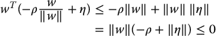
since ‖η‖ ⩽ ρ. Therefore
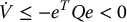
and the result follows. Finally, note from Equation (9.67) that ‖δa‖ ⩽ ρ as required.
Since the above control term δa is discontinuous on the subspace defined by BTPe = 0, solution trajectories on this subspace are not well defined in the usual sense. One may define solutions in a generalized sense, the so-called Filippov solutions [46]. In practice, the discontinuity in the control results in the phenomenon of chattering, where the control switches rapidly between the control values in (9.63).
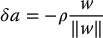
To avoid control chattering, we may implement a continuous approximation to the above discontinuous control as
In this case, since the control signal given by Equation (9.70) is continuous and differentiable except at ‖BTPe‖, a solution to the system (9.52) exists for any initial condition and we can prove the following result.
Theroem 9.1.
All trajectories of the system (9.52) are uniformly ultimately bounded (u.u.b.) using the continuous control law (9.70). (See Appendix C for the definition of uniform ultimate boundedness.)
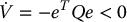
Proof: As before, choose V(e) = eTPe and compute
with ‖w‖ = ‖BTPe‖ as above. For ‖w‖ ⩾ ε the argument proceeds as above and  . For ‖w‖ ⩽ ε the second term in (9.72) becomes
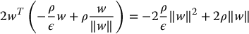
This expression attains a maximum value of  when
when  . Thus, we have
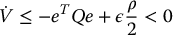
provided

Using the relationship (see B.5)

from Equation (B.5), where λmin(Q), λmax(Q) denote the minimum and maximum eigenvalues, respectively, of the matrix Q, we have that  if
if
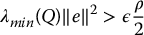
or, equivalently
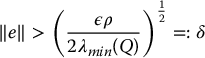
Let Sδ denote the smallest level set of V containing B(δ), the ball of radius δ and let Br denote the smallest ball containing Sδ. Then all solutions of the closed-loop system are u.u.b. with respect to Br. The situation is shown in Figure 9.3. All trajectories will eventually reach the boundary of Sδ since  is negative definite outside of Sδ and hence remain inside the ball Br.

Figure 9.3 The uniform ultimate boundedness set. Since  is negative outside the ball Bδ, all trajectories will eventually enter the level set Sδ, the smallest level set of V containing Bδ. The system is thus u.u.b. with respect to Br, the smallest ball containing Sδ.
Note that the radius of the ultimate boundedness set, and hence, the magnitude of the steady-state tracking error, is proportional to the product of the uncertainty bound ρ and the constant ε.
9.3.4 Adaptive Inverse Dynamics
This section is concerned with the adaptive control problem in which an estimation scheme is used to generate estimated values of parameters that are then used in lieu of the true parameters.
Once the linear parametrization property for manipulators became widely known in the mid-1980’s, the first globally convergent adaptive control results began to appear. These first results were based on the inverse dynamics approach discussed above. Consider the plant given by Equation (9.44) and the control given by Equation (9.45) as above, but now suppose that the parameters appearing in Equation (9.45) are not fixed as in the robust control approach, but are time-varying estimates of the true parameters. Substituting Equation (9.45) into Equation (9.44) and setting

it can be shown (Problem 9–11), using the linear parametrization property, that

where  is the regressor function defined in Equation (6.122) and
  , where
  is the estimate of the parameter vector θ. In state space we write the system (9.79) as
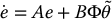
where
with K0 and K1 chosen as before as diagonal matrices of positive gains so that A is a Hurwitz matrix. Let P be the unique symmetric, positive definite matrix P satisfying the matrix Lyapunov equation
and choose the parameter update law as
where Γ is a constant, symmetric, positive definite matrix. Then, global convergence to zero of the tracking error with all internal signals remaining bounded can be shown using the Lyapunov function
To see this we calculate  as (Problem 9–12)

the latter term following since θ is constant, that is,  . Using the parameter update law (9.83) we have
Remark 9.2.
It is important to understand why the Lyapunov function V in Equation (9.86) is only negative semi-definite whereas V in Equation (9.69) is negative definite. In the robust approach the states of the system are  and
and  . In the adaptive control approach, the fact that
  satisfies the differential equation (9.83) means that the complete state vector now includes
  and the state equations are given by the coupled system, Equations (9.80) and (9.83). For this reason we included the positive definite term
  in the Lyapunov function (9.84).
From Equation (9.86) it follows that the position tracking errors converge to zero asymptotically and the parameter estimation errors  remain bounded. We will not go through the details of the proof in this section. The argument is similar to that of the passivity-based, adaptive control approach of the next section so we will defer the details until later. In order to implement this adaptive inverse dynamics scheme, however, one notes that the acceleration
  is needed in the parameter update law and that
  must be invertible. The need for the joint acceleration in the parameter update law presents a serious challenge to its implementation. Acceleration sensors are noisy and introduce additional cost whereas calculating the acceleration by numerical differentiation of position or velocity signals is not feasible in most cases. The invertibility of
  can be enforced in the algorithm by resetting the parameter estimate whenever
  would otherwise result in
  becoming singular. The passivity-based approaches that we treat next remove both of these impediments.
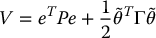
9.4 Passivity-Based Control
The inverse dynamics based approaches in the previous section rely, in the ideal case, on exact cancellation of all nonlinearities in the system dynamics. In this section we discuss control techniques based on the passivity or skew symmetry property of the Euler–Lagrange equations. These methods do not rely on complete cancellation of nonlinearities and hence, do not lead to a linear closed-loop system even in the known-parameter case. However, as we shall see, the passivity-based methods have other advantages with respect to robust and adaptive control.
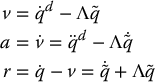
To motivate the discussion to follow, consider again the Euler–Lagrange equations

and choose the control input according to

where the quantities v, a, and r are given as

where K and Λ are diagonal matrices of constant, positive gains. Substituting the control law (9.88) into the plant model (9.87) leads to

Note that, in contrast to the inverse dynamics control approach, the closed-loop system (9.90) is still a coupled nonlinear system. Stability and asymptotic convergence of the tracking error to zero therefore are not obvious and require additional analysis.
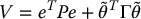
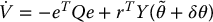
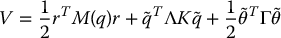
Consider the Lyapunov function candidate
Calculating  yields
Using the skew symmetry property and the definition of r, Equation (9.92) reduces to
where
Therefore the equilibrium e = 0 in error space is globally asymptotically stable.
In fact, assuming constant norm bounds on the inertia matrix M(q), it is fairly straightforward to prove global exponential stability of the tracking error. In the case of the inverse dynamics control considered previously, we concluded exactly the same result in a much simpler way. Therefore the advantages, if any, of the passivity-based control over the inverse dynamics control are unclear at this point. We will see in the next two sections that the real advantage of the passivity-based approach occurs for the robust and adaptive control problems. In the robust control approach considered next we will see that the assumption  can be eliminated and that the computation of the uncertainty bounds is greatly simplified. In the adaptive control approach we will see that the requirements on acceleration measurement and boundedness of the estimated inertia matrix
  can be eliminated. Thus, the passivity-based approach has some very important advantages over the inverse dynamics approach for the robust and adaptive control problems.
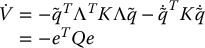
9.4.1 Passivity-Based Robust Control
In this section we use the passivity-based approach above to derive an alternative robust control algorithm that exploits both the skew symmetry property and linearity in the parameters and leads to a much easier design in terms of computation of uncertainty bounds. We modify the control input (9.88) as

where K, Λ, v, a, and r are given by (9.89). In terms of the linear parametrization of the robot dynamics, the control (9.95) becomes
and the combination of Equation (9.95) with Equation (9.87) yields

We now choose the term  in Equation (9.96) as

where θ0 is a fixed nominal parameter vector and δθ is an additional control term. The system (9.97) then becomes

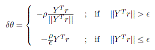
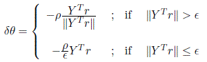
where  is a constant vector and represents the parametric uncertainty in the system. If the uncertainty can be bounded by finding a nonnegative constant ρ ⩾ 0 such that
then the additional term δθ can be designed according to
Using the same Lyapunov function candidate from Equation (9.91) above, we can show uniform ultimate boundedness of the tracking error. Carrying out the details of the calculation of  yields
Uniform ultimate boundedness of the tracking error follows with the control δθ from Equation (9.101) exactly as in the proof of Theorem 9.5. The details are left as an exercise (Problem 9–14).
Comparing this approach with the approach in Section 9.3.3 we see that finding a constant bound ρ for the constant vector  is much simpler than finding a time-varying and state-dependent bound for η in Equation (9.47). The bound ρ in this case depends only on the inertia parameters of the manipulator, while ρ(x, t) in Equation (9.54) depends on the manipulator state vector, the reference trajectory and, in addition, requires some assumptions on the estimated inertia matrix
  .
.
9.4.2 Passivity-Based Adaptive Control
In the adaptive approach the vector  in Equation (9.96) is taken to be a time-varying estimate of the true parameter vector θ. Combining the control law, Equation (9.95), with Equation (9.87) yields

The parameter estimate  may be computed using standard methods of adaptive control such as gradient or least squares. For example, using the gradient update law

together with the Lyapunov function
results in global convergence of the tracking errors to zero and boundedness of the parameter estimates. Computing  along trajectories of the system (9.103), we obtain

Substituting the expression for  from the gradient update law (9.104) into Equation (9.106) yields

where e and Q are defined as before, showing that the closed-loop system is stable in the sense of Lyapunov. It follows that the tracking error e(t) converges asymptotically to zero and the estimation error  is bounded. In order to show this we note that since
  is nonincreasing from Equation (9.107), the value of V(t) can be no greater than its value at t = 0. Since V consists of a sum of nonnegative terms, this means that each of the terms r,
  , and
, and  are bounded as functions of time.
With regard to the tracking error,  ,
,  , we also note that
  is quadratic in the error vector e(t). Integrating both sides of Equation (9.107) gives
As a consequence, the tracking error vector e(t) is a square integrable function. Such functions, under some mild additional restrictions, must tend to zero as t → ∞. Specifically, we may appeal Barbalat’s Lemma
from Appendix C. Since both  and
and  have already been shown to be bounded, it follows that
  is also bounded. Therefore, we have that
  is square integrable and its derivative is bounded. Hence, the tracking error
  as t → ∞.
To show that the velocity tracking error also converges to zero, one must appeal to the equations of motion (9.103), from which one may argue that the acceleration  is bounded. It follows that the velocity error
  asymptotically converges to zero provided that the reference acceleration
  is bounded.
9.5 Torque Optimization
In previous sections we considered the effect of parameter uncertainty in the design of control laws for n-link manipulators and derived both robust and adaptive control schemes to deal with uncertain or unknown inertia parameters. In this section we consider the problem of actuator saturation in the design of nonlinear control laws. Actuator saturation, together with joint elasticity and friction, have long been recognized as the primary factors that limit the performance of manipulators. Actuator saturation may be considered as part of the motion planning problem, for example, by including bounds on the velocities and accelerations when planning desired trajectories and then correlating these bounds with bounds on the actuator torques.
In this section we discuss an alternative method that views the problem of designing a nonlinear control law subject to actuator saturation as a constrained torque optimization problem. Given a nominal control law designed as a first step without considering input constraints, the goal is to find a control law “closest” to the nominal control with respect to a given norm. The optimal control is thus determined by solving a quadratic programming problem at each time step.
Consider again the Euler–Lagrange equations for an n-link manipulator

and suppose that the torque input u = (u1, ⋅⋅⋅, un) is bounded as

For simplicity we will assume that these bounds are constant.
Example 9.1.
Consider the two-link, planar RR manipulator example from Section (6.4) and suppose that the nominal control law u0 is chosen as an inverse dynamics control (9.23)

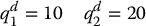
where qd(t) is the reference trajectory. For simplicity, we will take qd as a constant step change in the joint angles in this example so that
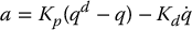
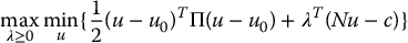
Figure (9.4) shows the joint responses with and without torque saturation, where we have taken

We see that the actual step responses deviate considerably from the ideal (unconstrained) responses with both overshoot and undershoot.

Figure 9.4 Joint responses and input torques with saturated and unsaturated inverse dynamics control.
Next, note that the inequality constraints (9.110) can be written as

where  and
and  are given by
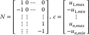
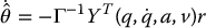
Let u0 be a control law designed by any method discussed so far, such as an inverse dynamics control, robust control, adaptive control, and so on. The torque optimization problem that we consider is then to choose the actual control input u to satisfy
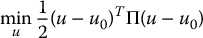
where Π is a symmetric, positive definite n × n matrix to be chosen by the designer. Note that Π need not necessarily be a constant matrix. Thus the minimization (9.117)–(9.118) is a quadratic programming that is solved pointwise, i.e. at each instant of time t.
The optimization problem (9.117)–(9.118) is called the primal problem. The primal problem can be shown to be equivalent to the optimization problem
where  is a vector of Lagrange multipliers.
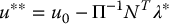
From (9.119) we see that the minimization over u is unconstrained. Therefore, after a straightforward calculation the minimizer u* is given by
Substituting u* from (9.120) back into (9.119) we get
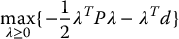
or equivalently
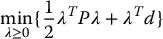
where
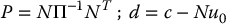
The minimization problem (9.122) is called the dual problem. Note that the dual problem is also a quadratic program.
Solving the dual problem for λ = λ* gives the optimal control input u** as

The advantage of the primal-dual method is that the dual problem has only the constraint λ ⩾ 0 and is therefore often easier to solve than the primal problem.
Example 9.2.
Going back to the previous example, with u0 given as an inverse dynamics control

if we choose Π in (9.117) as

where Q is a constant symmetric positive definite n × n matrix, then the optimal control law u** can be written as

Therefore we see that the optimization strategy amounts to modifying the outer-loop control term to account for the actuator saturation. This significance of this result is that the nominal inner-loop control remains unchanged and therefore we may incorporate the above torque optimization method into any control design methodology.
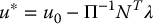
Figure (9.5) shows the joint responses and joint torques using the control law (9.128) computed by solving the dual problem. The tracking performance of the unconstrained control is nearly recovered.

Figure 9.5 Optimal joint trajectories and input torques using (9.128) compared with the unsaturated case.
9.6 Chapter Summary
In this chapter we discussed the nonlinear control problem for robot manipulators. We developed models of both rigid and flexible-joint robots. We then developed several control algorithms and discussed pros and cons of each as well as implementation aspects. Among the algorithms we discussed were PD control, inverse dynamics, and passivity-based control. Moreover we showed how to formulate robust and adaptive versions of the latter two approaches.
The rigid and flexible-joint robot models are, respectively:

A PD control law in joint space is of the form

Global asymptotic tracking for the rigid model can be shown using the Lyapunov function candidate below together with LaSalle’s theorem in case the gravity vector g(q) = 0.

PD Control with Gravity Compensation
With gravity present, the PD plus gravity compensation algorithm below also results in global asymptotic tracking for the rigid model.
The inverse dynamics control law consists of the following two expressions, the first being the inner-loop control and the second being the outer-loop control.

The inverse dynamics algorithm results in a closed-loop system that is linear and decoupled.
We showed that the modified outer-loop term below results in a linear, decoupled system in task space coordinates  , where X is a minimal representation of SE(3) and J is the analytical Jacobian.
We presented a Lyapunov-based approach for robust inverse dynamics control.

where  ,
,  , and
, and  are the nominal values of M, C, and g. From this we derived the state space model
where η represents the uncertainty resulting from inexact cancellation of nonlinearities and
The additional control input δa was chosen as
and shown to achieve uniform ultimate boundedness of the tracking errors. This is a practical notion of asymptotic stability in the sense that the tracking errors can be made small.
The adaptive version of the inverse dynamics control results in a system of the form
where θ represents the unknown parameters (masses, moments of inertia, etc.) The second equation above is used to estimate the parameters online. The Lyapunov function candidate below can be used to show asymptotic convergence of the tracking errors to zero and boundedness of the parameter estimation error.
Passivity-Based Robust Control
We introduced the notion of passivity-based control as an alternative to inverse dynamics control. This approach exploits the passivity property of the robot dynamics rather than attempting to cancel the nonlinearities as in the inverse dynamics approach. We presented a control algorithm of the form

where the quantities v, a, and r are given as
and K is a diagonal matrix of positive gains. This results in a closed-loop system

In the robust passivity-based approach the term  is chosen as

where θ0 is a fixed nominal parameter vector and δθ is an additional control term. The additional term δθ can be designed according to
where ρ is a bound on the parameter uncertainty. Uniform ultimate boundedness of the tracking errors follows using the Lyapunov function candidate

Passivity-Based Adaptive Control
In the adaptive version of this approach we derived the system
and used the Lyapunov function candidate

to show global convergence of the tracking errors to zero and boundedness of the parameter estimates.
Finally, we considered the problem of actuator saturation and formulated an optimization method to reduce the tracking errors caused by the input saturation. Given a nominal control u0, computed using any of the methods in this chapter, the actual control u is computed as a solution of a pointwise quadratic programming problem
where the constraints Nu ⩽ c account for the constraints on the input torque. We showed that the implementation of the above torque optimization requires only the modification of the outer-loop control term.
Problems
- Verify the properties of skew symmetry, passivity and linearity in the parameters for the system given by Equation (9.6). Compute bounds on the inertia matrix, M(q), in terms of bounds on D(q). Show that M(q) is positive definite.
- Form the Lagrangian for an n-link manipulator with joint flexibility using Equations (9.15) and (9.16). From this derive the equations of motion (9.18).
- Complete the proof of stability of PD control for the flexible-joint robot without gravity terms using the Lyapunov function candidate (9.20) and LaSalle’s theorem. Show that q1 = q2 in the steady state.
- Given the flexible-joint model defined by Equation (9.18) with the PD control law (9.19), what are the steady-state values of q1 and q2 if the gravity term is present? How could one define the reference angle qd in the case that gravity is present?
- Suppose that the PD control law given by Equation (9.19) is implemented using the link variables
where
 . Show that the equilibrium
  is unstable. Hint: Use Lyapunov’s First Method, that is, show that the equilibrium is unstable for the linearized system.
 - Simulate an inverse dynamics control law for a two-link elbow manipulator whose equations of motion were derived in Chapter 6. Investigate what happens if there are constraints on the input torque.
- For the system of Problem 9–6, what happens to the response of the system if the coriolis and centrifugal terms are dropped from the inverse dynamics control law in order to facilitate computation? What happens if incorrect values are used for the link masses? Investigate via computer simulation.
- Carry out the details to derive the uncertain system (9.46) and (9.47).
-
Consider the two-link RP manipulator shown in Figure 9.6.
Show that the rotational inertial about the first link is not bounded as a function of the prismatic joint variable d2. Discuss the implications of this for the problem of robust control. - Add an outer-loop correction term δa to the control law of Problem 9–7 to overcome the effects of uncertainty. Base your design on the second method of Lyapunov as in Section 9.3.3.
- Derive the error equation (9.79) using the linearity-in-the-parameters property of the robot dynamics.
- Verify the expression for
 in Equation (9.85).
 - Consider the coupled nonlinear system
where u1, u2 are the inputs and y1, y2 are the outputs.
- What is the dimension of the state space?
- Choose state variables and write the system as a system of first order differential equations in state space.
- Find an inverse dynamics control so that the closed-loop system is linear and decoupled, with each subsystem having natural frequency 10 radians and damping ratio 1/2.
- Complete the proof of uniform ultimate boundedness for the passivity-based robust control law given by Equation (9.95) applied to the rigid robot model.
- Prove the inequality (9.59).

Figure 9.6 Two-link RP manipulator.
Notes and References
Many of the fundamental theoretical problems in motion control of robot manipulators were solved during an intense period of research from about the mid-1980’s until the early-1990s, during which time researchers first began to exploit the structural properties of manipulator dynamics such as feedback linearizability, skew symmetry and passivity, multiple time-scale behavior, and other properties. For a more advanced treatment of some of these topics, the reader is referred to [167] and [32].
In the area of PD and PID control of manipulators, the earliest results are contained in [174]. These results were based on the Hamiltonian formulation of robot dynamics and effectively exploited the passivity property. The use of energy as a Lyapunov function is described in [78].
The problem of joint flexibility was first brought to the forefront of robotics research in [128], [172], and [173]. The model presented here to describe the dynamics of flexible-joint robots is due to [165].
The earliest results on computed torque appeared in [110] and [136]. A related approach known as the method of resolved motion acceleration control is due to [104]. In [83] these various control schemes are all compared to the method of inverse dynamics and shown to be essentially equivalent.
The robust inverse dynamics control approach here follows closely the general methodology in [28]. The earliest application of this method to the manipulator control problem was in [31] and [168]. This technique is closely related to the so-called method of sliding modes, which has been applied to manipulator control in [154]. A very complete survey of robust control of robots up to about 1990 is found in [1]. Other results in robust control from an operator theoretic viewpoint are [170] and [58]. The passivity-based robust control result here is due to [166].
The question of when the inertia matrix of a robot manipulator is bounded is treated in detail in [53].
The adaptive inverse dynamics control result presented here is due to [29]. Other notable results in this area appeared in [114]. The first results in passivity-based adaptive control of manipulators was in [67] and [153]. The Lyapunov stability proof presented here is due to [161]. A unifying treatment of adaptive manipulator control from a passivity perspective was presented in [131]. Other works based on passivity are [19] and [12].
One of the problems with the adaptive control approaches considered here is the so-called parameter drift problem. The Lyapunov stability proofs presented show that the parameter estimates are bounded but there is no guarantee that the estimated parameters converge to their true values. It can be shown that the estimated parameters converge to the true parameters provided the reference trajectory satisfies the condition of persistency of excitation
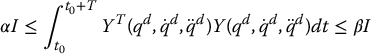
for all t0, where α, β, and T are positive constants.
 means that the expression is identically equal to zero, not simply zero at one instant of time.