CHAPTER 8
INDEPENDENT JOINT CONTROL
8.1 Introduction
The control problem for robot manipulators is to determine the time history of joint inputs required to cause the end effector to execute a commanded motion. The joint inputs may be joint forces and torques, or they may be inputs to the actuators, for example, voltage or current inputs to the motors, depending on the model used for controller design. The commanded motion is typically specified either as a sequence of end-effector positions and orientations, or as a continuous path.
There are many control techniques and methodologies that can be applied to the control of manipulators. The particular control method used can have a significant impact on the performance of the manipulator and consequently on the range of its possible applications. For example, continuous path tracking requires a different control architecture than does point-to-point motion.
In addition, the mechanical design of the manipulator itself will influence the type of control scheme needed. For example, the control problems encountered with a Cartesian manipulator are different from those encountered with an elbow manipulator. This creates a so-called hardware/ software trade-off between the mechanical structure of the system and the architecture/programming of the controller.
Technological improvements are continually being made in the mechanical design of robots, which in turn improves their performance potential and broadens their range of applications. Realizing this increased performance, however, requires more sophisticated approaches to control. One can draw an analogy to the aerospace industry. Early aircraft were relatively easy to fly but possessed limited performance capabilities. As performance increased with technological advances, so did the problems of control to the extent that the latest vehicles, such as the space shuttle or forward swept wing fighter aircraft, cannot be flown without sophisticated computer control.
As an illustration of the effect of the mechanical design on the control problem, we may compare a robot actuated by permanent magnet DC motors with gear reduction to a direct-drive robot using high-torque motors with no gear reduction. In the first case, the motor dynamics are linear and well understood and the effect of the gear reduction is largely to decouple the system by reducing the inertia coupling among the joints. However, the presence of the gears introduces friction, drive train compliance, and backlash.
In the case of a direct-drive robot, the problems of backlash, friction, and compliance due to the gears are eliminated. However, the inertia coupling among the links is now significant, and the dynamics of the motors themselves may be much more complex. The result is that in order to achieve high performance from this type of manipulator, a different set of control problems must be addressed.
In this chapter we consider the simplest type of control strategy, namely, independent joint control. In this type of control each axis of the manipulator is controlled as a single-input/single-output (SISO) system. Any coupling effects due to the motion of the other links are treated as disturbances.
The basic structure of a single-input/single-output feedback control system is shown in Figure 8.1.

Figure 8.1 Basic structure of a feedback control system. The compensator measures the error between a reference and a measured output and produces signals to the plant that are designed to drive the error to zero despite the presence of disturbances.
The design objective is to choose the compensator in such a way that the plant output follows or tracks a desired output, given by the reference signal. The control signal, however, is not the only input acting on the system. Disturbances, which are really inputs that we do not control, also influence the behavior of the output. Therefore, the controller must be designed, in addition, so that the effects of the disturbances on the plant output are reduced. If this is accomplished, the plant is said to reject the disturbances. The twin objectives of tracking and disturbance rejection are central to any control methodology.
8.2 Actuator Dynamics
Robot manipulators are equipped with actuators to move the joints through programmed motion trajectories in order to complete given tasks. These actuators may be electric, hydraulic, or pneumatic. In this section we restrict our attention to the dynamics of permanent magnet DC motors, as these are the simplest actuators to analyze and are commonly used in robot manipulators. Other types of electric motors, in particular AC motors and so-called brushless DC motors, are also used as actuators for robots but we will not discuss their dynamics here.
A DC motor works on the principle that a current-carrying conductor in a magnetic field experiences a force F = i × ϕ, where ϕ is the magnetic flux, i is the current in the conductor, and × is the vector cross product. The motor itself consists of a fixed stator and a movable rotor that rotates inside the stator as shown in Figure 8.2.

Figure 8.2 Principle of operation of a permanent magnet DC motor. The magnitude of the force (or torque) on the armature is proportional to the product of the current and magnetic flux. A commutator is required to periodically switch the direction of the current through the armature to keep it rotating in the same direction.
If the stator produces a radial magnetic flux ϕ and the current in the rotor (also called the armature) is i, then there will be a torque on the rotor causing it to rotate. The magnitude of this torque is

where τm is the motor torque (Newton-meters), ϕ is the magnetic flux (webers), ia is the armature current (amperes), and K1 is a physical constant.
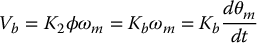
In addition, whenever a conductor moves in a magnetic field, a voltage Vb is generated across its terminals that is proportional to the velocity of the conductor in the field. This voltage, called the back emf, will tend to oppose the current flow in the conductor. Thus, in addition to the torque τm in Equation (8.1), we have the back emf relation
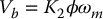
where Vb denotes the back emf (volts), ωm is the angular velocity of the rotor (radians per second), and K2 is a proportionality constant.
DC motors can be classified according to the way in which the magnetic field is produced and the armature is designed. Here we discuss only the so-called permanent magnet motors whose stator consists of a permanent magnet. In this case we can take the flux ϕ to be a constant. The torque on the rotor is then controlled by controlling the armature current ia.
Consider the schematic diagram of Figure 8.3, where

Figure 8.3 Circuit diagram for an armature controlled DC motor. The rotor windings have an effective inductance L and effective resistance R. The applied voltage V is the control input.
The differential equation for the armature current is then
Since the flux ϕ is constant, the torque developed by the motor is
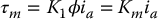
where Km is the torque constant in N-m/amp. Also, from Equation (8.2) we have
where Kb is the back emf constant. It can be shown that the numerical values of Km and Kb are the same provided MKS units1 are used.
The torque constant can be determined from a set of torque-speed curves as shown in Figure 8.4 for various values of the applied voltage V.

Figure 8.4 Typical torque-speed curves of a DC motor. Each line represents the torque versus speed for a given value of the applied voltage.
When the motor is stalled, the blocked-rotor torque at the rated voltage Vr is denoted by τ0. Using Equations (8.3) and (8.4) with Vb = 0 and dia/dt = 0 we have
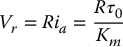
Therefore the torque constant is

8.3 Load Dynamics
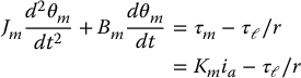
In this section we consider the dynamics of the DC motor in series with a gear train and load as shown in Figure 8.5. The gear ratio is r: 1, where r typically has values in the range 20 to 200 or more. The load is represented by the rotational inertia Jℓ. Referring to Figure 8.5, we set Jm = Ja + Jg, the sum of the actuator and gear inertias.

Figure 8.5 Lumped model of a single link with actuator and gear train. Ja, Jg, and Jℓ are, respectively, the actuator, gear, and load inertias. Bm is the coefficient of motor friction and includes friction in the brushes and gears. The gear ratio is r: 1 with r ≫ 1.
In terms of the motor angle θm, the equation of motion of this system is then
the latter equality coming from Equation (8.4). In the Laplace domain the three Equations (8.3), (8.5), and (8.8) may be combined and written as


The block diagram of the above system is shown in Figure 8.6.

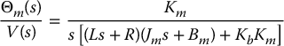
Figure 8.6 Block diagram for a DC motor system. The block diagram represents a third-order system from input voltage V(s) to output position θm(s).
The transfer function from V(s) to Θm(s) is given, with τℓ = 0, by (Problem 8–1)
The transfer function from the load torque τℓ(s) to Θm(s) is given, with V = 0, by (Problem 8–1)
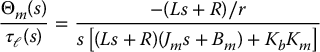
Notice that the magnitude of this latter transfer function, and hence the effect of the load torque on the motor angle, is reduced by the gear ratio r.
Frequently it is assumed that the “electrical time constant” L/R is much smaller than the “mechanical time constant” Jm/Bm. This is a reasonable assumption for many electromechanical systems and leads to a reduced order model of the actuator dynamics. If we divide numerator and denominator of Equations (8.11) and (8.12) by R and neglect the electrical time constant by setting L/R equal to zero, the transfer functions in Equations (8.11) and (8.12) become, respectively, (Problem 8–2)

and

In the time domain Equations (8.13) and (8.14) represent, by superposition, the second-order differential equation

The block diagram corresponding to the reduced-order system (8.15) is shown in Figure 8.7.

Figure 8.7 Block diagram for the reduced-order system. The block diagram now represents a second-order system.
8.4 Independent Joint Model
In this section we refine the previous model by assuming that the load attached to the DC motor is a link of a multi-link manipulator rather than a simple rotational inertia in order to generate a more accurate description of the manipulator load dynamics. This section assumes knowledge of the Euler–Lagrange equations that we derived in Chapter 6 and may be skipped if the reader has not studied that chapter.
In Chapter 6 we obtained the following set of differential equations describing the motion of an n-degree-of-freedom manipulator (cf. Equation (6.66))

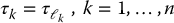
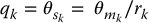
We assume that the k-th component, τk, of the generalized force vector τ is a torque about the axis zk − 1 if joint k is revolute, and is a force along zk − 1 if joint k is prismatic. If the output side of the gear train is directly coupled to the joint axis, then the joint variables and motor variables are related by

where rk is the k-th gear ratio. Similarly, the joint torques τk given by (8.16) and the actuator load torques  are related by
Remark 8.1.
In many manipulator designs, such as those incorporating belts, pulleys or chains between the actuators and joints the relationship between joint variables and actuator variables is more complicated. In general, one must incorporate a transformation of the form

where  .
.
Example 8.1.
Consider the two-link manipulator shown in Figure 8.8 whose actuators are both located on the robot base. In this case we have


Figure 8.8 Two-link manipulator with remotely driven link.
For the following discussion, assume for simplicity that the joint variables qk,  and actuator variables
  , τk are related as follows

Then the equations of motion of the manipulator can be written componentwise, for k = 1, …, n as
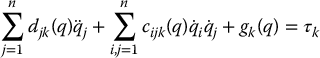

Equation (8.25) represents the actuator dynamics and Equation (8.24) represents the nonlinear inertial, centripetal, coriolis, and gravitational coupling effects due to the motion of the manipulator. The simplest approach to the control of the above system is to consider the nonlinear term τk entering (8.25) and defined by (8.24) as an input disturbance to the motor and design an independent controller for each joint according to the model (8.25). The advantage of this approach is its simplicity since the motor dynamics represented by (8.25) are linear. Note that the term τk in (8.25) is divided by the gear ratio rk. This is an important observation. The effect of the gear reduction is to reduce magnitude of the coupling nonlinearities given by (8.24), which adds to the validity of the independent joint control approach. However, for very high speed motion or for direct-drive manipulators without gear reduction at the joints, the coupling nonlinearities have a much larger effect on the performance of the system and so treating the nonlinear coupling effects as a disturbance will generally result in larger tracking errors. For this reason, we will introduce more advanced, nonlinear feedback control methods in Chapter 9.
Now, since  , the actual coefficient of
  in (8.25), includes the term dkk(q)/r2k from (8.24) and is thus given by

which is, of course, configuration dependent and may vary over a large range. For example, Figure 8.9 shows the approximate range of inertias for the Stanford manipulator from [11].

Figure 8.9 Approximate range of effective inertias Jkk for the Stanford manipulator (kgm2) from [11].
Therefore, we may approximate the inertia coefficient Jkk by a constant average or effective inertia, called  , for example, by taking the midpoint of values such as those in Table 8.9.
Setting

we write Equation (8.25) as
where dk is treated as a disturbance and defined by
Note that both Equations (8.15) and (8.28) are of the form

for suitable definitions of J and B and where u(t) is a control input with units of torque and d(t) represents a disturbance torque. Henceforth we will use this model (8.30) in the subsequent discussion of the compensator design. The block diagram in the Laplace domain corresponding to the reduced-order system (8.30) is shown in Figure 8.10.

Figure 8.10 Block diagram of the simplified, open-loop system. The disturbance d/r represents all of the nonlinearities and coupling from the other links.
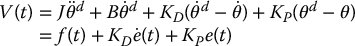
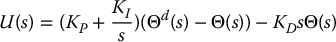
8.5 PID Control
The PID (Proportional, Integral, Derivative) compensator is the most common type of controller used in most manipulators. The general form of a PID controller u(t) is

where e(t) = θ(t) − θd(t) is the tracking error. The controller parameters are the proportional gain KP, integral gain KI, and derivative gain KD. In the Laplace domain we write Equation (8.31) as

and we call
the PID compensator.
Referring to Equation (8.33), the PID Compensator adds a pole (at s = 0) and two zeros (roots of KDs2 + KPs + KI) to the forward transfer function. The design problem, known as tuning, is then to choose the PID gains KP, KD, and KI to achieve the desired performance. There are numerous results available for tuning PID compensators and we will not repeat them in any detail. The goal here is to provide insight into some of the main practical problems that arise in compensator design for a single link of a robot manipulator.
Two-Degree-of-Freedom Controller
In Figure 8.11, the compensator acts on the error signal. If the reference θd is a step reference, then the derivative term will introduce an impulse at t = 0. To avoid this we may use the alternative architecture shown in Figure 8.12, which is often called a two-degree-of-freedom controller. In this architecture, the input to the derivative term KDs is the output signal θ, rather than the error signal θ − θd, which avoids differentiating the step input θd at time t = 0, where the step function is discontinuous.

Figure 8.11 The system in Figure 8.10 with a PID compensator. KP, KI and KD are the proportional, integral and derivative gains and Θd is the joint angle reference signal to be tracked.

Figure 8.12 The system in Figure 8.10 with a two-degree-of-freedom PID compensator.
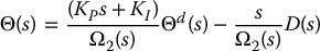
Whether we use the controller configuration in Figure 8.11 or Figure 8.12, we must analyze the appropriate transfer functions to assess the performance of the closed-loop systems. The transfer functions of relevance are, in each case,  , the transfer function from the reference to the output, and
  , the transfer function from the disturbance to the output.
The transfer function G1(s) is computed by setting the disturbance input D(s) equal to zero. Likewise, the transfer function G2(s) is computed by setting the reference input Θd(s) equal to zero. By the Principle of Superposition then, the overall system response, in each case, is given by
The first two rows in Table 8.1 show the four closed-loop transfer functions from the reference input Θd(s) to the output Θ(s) (G1(s)) with the one- and two-degree-of-freedom architectures for both PID and PD compensators. The third row in Table 8.1 shows corresponding closed-loop transfer functions from the disturbance input D(s) to the output Θ(s) (G2(s)). In the latter case, the transfer functions from D(s) to Θ(s) are the same for both the one- and two-degree-of-freedom architectures. The derivation of these transfer function is straigt!forward and left as an exercise (Problem 8–4).
Remark 8.2. (Derivative Filter).
Note that the derivative term KDs in the PID compensator involves differentiation of the signal θ(t). In practice, a differentiator will amplify high-frequency signals and thus will perform poorly in the presence of noise. One may avoid using a pure differentiator by using a velocity sensor, such as a tachometer, to measure  directly or, more commonly, to use a filter of the form
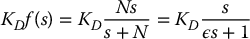
where ε = 1/N. Note that f(s) → s, an ideal differentiator, as ε → 0 and thus represents an approximate differentiator for small values of ε and low frequencies in s. The effect of such a derivative filter is both to introduce phase lag into the estimate of  but also to mitigate the effect of noise amplification caused by ideal differentiation.
Table 8.1 Closed-loop transfer functions using both the one- and two-degree-of-freedom architectures. a) and d) represent G1(s) in the one-degree-of-freedom architecture. b) and e) represent G1(s) in the two-degree-of-freedom architecture. c) and f) represent G2(s).
| With PID Compensator | With PD Compensator |
a) 
|
d) 
|
b) 
|
e) 
|
c) 
|
f) 
|
In this section, we consider the problem of set-point tracking, which is the problem of tracking a constant or step reference command θd and arises in point-to-point motion. Since the reference input is a step signal, we will use the two-degree-of-freedom compensator in Figure 8.12.
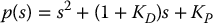
We first consider a PD compensator by setting the integral gain KI equal to zero. In this case, we see from Table 8.1 that the closed-loop system is given by

where Ω(s) is the closed-loop characteristic polynomial

The closed-loop system will be stable for all positive values of KP and KD and bounded disturbances, and the tracking error E(s) is given by

For a step reference input

and a constant disturbance

it follows directly from the final value theorem that the steady-state error ess satisfies
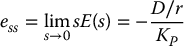
Since the magnitude of the disturbance is proportional to the gear ratio 1/r, we see that the steady state error is smaller for larger gear ratio and can be made arbitrarily small by making the position gain KP large, which is to be expected since the system is type 1.
Using a PD compensator, the closed-loop system is second-order and hence the step response is determined by the closed-loop natural frequency ω and damping ratio ζ. Given a desired value for these quantities, the gains KD and KP can be found from the expression
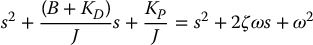
as
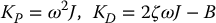
It is customary in robotics applications to take the damping ratio ζ = 1 so that the response is critically damped. In this context ω determines the speed of response.
Example 8.2.
Taking J = B = 1, for illustrative purposes, the closed-loop characteristic polynomial is
With θd = 1 and no disturbance acting on the system, Figure 8.13(a) shows the resulting step responses for several values of the natural frequency ω. If there is a constant disturbance, we recall from Equation (8.40) that there will be a steady-state error  . This steady-state error can be reduced by increasing the proportional gain Kp, but cannot be eliminated entirely for any finite KP. Figure 8.13(b) shows the steady-state error for the same values of ω.

Figure 8.13 Second-order step responses with PD control. The speed of response, as measured by rise time, is faster for larger values of the natural frequency ω. Likewise, the steady-state error due to a constant disturbance is smaller for larger values of ω.
In theory, an arbitrarily fast response and arbitrarily small steady-state error to a constant disturbance could be achieved by simply increasing the gains in the PD compensator. In practice, however, there is a maximum speed of response achievable from the system due to limits on the maximum torque (or current) saturation, due to limits on the maximum torque output of the motors. Many manipulators, in fact, incorporate current limiters in the servo-system to prevent damage to the motors that migt! result from overdrawing current.
Figure 8.14 therefore includes a saturation function represents the maximum allowable output of the compensator. Figure 8.15 shows a comparison of the step responses with and without saturation. The disturbance input has been set to zero.

Figure 8.14 Second-order system with input saturation limiting the magnitude of the input signal. Increasing the magnitude of the compensator output signal beyond the saturation limit will not increase the input to the plant.

Figure 8.15 Second-order step response with PD control and saturation.
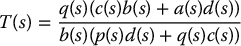
In order to remove the steady-state error due to the disturbance entirely we can employ integral control. Adding an integral term KI/s to the above results in the closed-loop transfer functions b) and c) in Table 8.1. The PID control achieves exact steady tracking of step inputs while rejecting step disturbances, provided of course that the closed-loop system is stable.
With the PID compensator

the closed-loop system is now the third order system
with characteristic polynomial

Applying the Routh–Hurwitz criterion to this polynomial, it follows that the closed-loop system is stable if the gains are positive, and in addition,

A common design rule-of-thumb for PID control is to first set KI = 0 and design the proportional and derivative gains, KP and KD, to achieve the desired transient behavior (rise time, settling time, and so forth) and then to choose KI within the limits imposed by (8.47) to remove the steady-state error.
Example 8.3.
To the previous system we have added an integral control term in the compensator. The step responses are shown in Figure 8.16. We see that the steady-state error due to the disturbance is removed.

Figure 8.16 Response with integral control action showing that the steady-state error to a constant disturbance has been removed.
8.6 Feedforward Control
The analysis in the previous section was carried out under the assumption that the reference signal and disturbance are constant and is not valid for tracking more general time-varying trajectories such as a cubic polynomial trajectory of the type generated in Chapter 7. In this section we introduce the notion of feedforward control as a method to track time-varying trajectories. We use the one-degree-off freedom architecture for simplicity.
8.6.1 Trajectory Tracking
Suppose that θd(t) is a joint space reference trajectory and consider the block diagram of Figure 8.17, where G(s) represents the forward transfer function of a given system and H(s) is the compensator transfer function.

Figure 8.17 Feedforward control scheme. F(s) is the feedforward transfer function which has the reference signal Θd as input. The output of the feedforward block is superimposed on the output of the compensator H(s).
A feedforward control scheme consists of adding a feedforward path with transfer function F(s) as shown. Let each of the three transfer functions be represented as ratios of polynomials
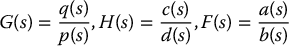
We assume that G(s) is strictly proper and H(s) is proper. Simple block diagram manipulation shows that the closed-loop transfer function  is given by (Problem 8–9)
The closed-loop characteristic polynomial is b(s)(p(s)d(s) + q(s)c(s)). Therefore, for stability of the closed-loop system, we require that the compensator H(s) and the feedforward transfer function F(s) be chosen so that the polynomials p(s)d(s) + q(s)c(s) and b(s) are Hurwitz. This says that, in addition to stability of the closed-loop system, the feedforward transfer function F(s) must itself be stable.
If we choose the feedforward transfer function F(s) equal to 1/G(s), the inverse of the forward plant, that is, a(s) = p(s) and b(s) = q(s), then the closed-loop system becomes

or, in terms of the tracking error E(s) = R(s) − Y(s),

Thus, assuming stability, the output θ(t) will track any reference trajectory θd(t). Note that we can only choose F(s) in this manner provided that the numerator polynomial q(s) of the forward plant is Hurwitz, that is, as long as all zeros of the forward plant are in the left half plane. Such systems are called minimum phase.
If there is a disturbance D(s) entering the system as shown in Figure 8.18, then it is easily shown (Problem 8–10) that the tracking error E(s) is given by
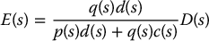

Figure 8.18 Feedforward control with disturbance D(s).
We have thus shown that, in the absence of disturbances, the closed-loop system will track any desired trajectory θd(t) provided that the closed-loop system is stable. The steady-state error is thus due only to the disturbance.
Let us apply this idea to the model of Section 8.5. Suppose that θd(t) is an arbitrary trajectory that we wish the system to track. In this case we have G(s) = 1/(Js2 + Bs) together with a PD compensator H(s) = KP + KDs.
We see that the plant transfer function G(s) has no finite zeros and hence is minimum phase. Thus, we can choose the feedforward transfer F(s) as F(s) = Js2 + Bs. The resulting system is shown in Figure 8.19.

Figure 8.19 Feedforward compensator for the second-order system of Section 8.5.
Note that 1/G(s) is not a proper rational function. However, since the derivatives of the reference trajectory θd(t) are known and precomputed, the implementation of the above scheme does not require differentiation of an actual signal. It is easy to see from Equation (8.52) that the steady-state error to a step disturbance is now given by the same expression as in Equation (8.40) independent of the reference trajectory. As before, a PID compensator would result in zero steady-state error to a step disturbance. In the time domain the control law of Figure 8.19 can be written as
where f(t) is the feedforward signal
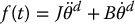
and e(t) is the tracking error θd(t) − θ(t). Since the forward plant equation is

the closed-loop error e(t) = θ(t) − θd(t) satisfies the second-order differential equation

We note from Equation (8.55) that the characteristic polynomial of the closed-loop system is identical to Equation (8.36). However, the system (8.55) is now written in terms of the tracking error e(t). Therefore, assuming that the closed-loop system is stable, the tracking error will approach zero asymptotically for any desired joint space trajectory in the absence of disturbances, that is, if d = 0.
8.6.2 The Method of Computed Torque
In this section we discuss the so-called method of computed torque, which as we shall see, can be viewed as a feedforward disturbance rejection scheme. This section assumes knowledge of the Euler–Lagrange equations from Chapter 6.
We see that the feedforward signal (8.54) results in asymptotic tracking of any trajectory in the absence of disturbances but does not otherwise improve the disturbance rejection properties of the system. However, although the term d(t) represents a disturbance, it is not completely unknown since d(t) satisfies (8.29). Thus we may consider adding to the above feedforward signal a term to anticipate and cancel the effects of the disturbance d(t). This is known as feedforward disturbance cancellation.
Consider the block diagram in Figure 8.20. Given desired trajectories qd(t) = (qd1(t), …, qnd(t)) for each joint and desired joint velocities and accelerations  and
and  , respectively, we superimpose the term ddk(t) at the k-th joint according to
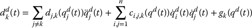

Figure 8.20 Computed torque feedforward disturbance cancellation. The term (8.56) is added to the output of the compensator to cancel the effect of the disturbance.
Since ddk(t) has units of torque, the above feedforward disturbance cancellation control is called the method of computed torque. The expression (8.56) compensates in a feedforward manner the nonlinear coupling inertia, Coriolis, centripetal, and gravitational forces arising from the motion of the manipulator.
8.7 Drive-Train Dynamics
A second effect that limits the achievable performance of a manipulator is flexibility in the motor shaft and/or drive train. We refer to this as joint flexibility or joint elasticity. For many manipulators, particularly those using so-called strain wave gears or harmonic gears, for torque transmission, the joint flexibility is significant. In addition to torsional flexibility in the gears, joint flexibility is caused by effects such as shaft windup, bearing deformation, and compressibility of the hydraulic fluid in hydraulic robots.
Remark 8.3.
Let kr be the effective stiffness at the joint. The joint resonant frequency is then  . It is common engineering practice to limit ω in Equation (8.42) to no more than half of ωr to avoid excitation of the joint resonance. However, in order to say more, we will model the flexibility and consider more advanced control design methods below.
Harmonic gears are a type of gear mechanism that are very popular for use in robots due to their low backlash, high torque transmission, and compact size.
A typical harmonic gear, the Harmonic Drive® gear, is shown in Figure 8.21 and consists of a rigid circular spline, a flexible flexspline, and an elliptical wave generator. The wave generator is attached to the actuator and hence is turned at high speed by the motor. The circular spline is attached to the load. As the wave generator rotates it deforms the flexspline causing a number of teeth of the flexspline to mesh with the teeth of the circular spline. The effective gear ratio is determined by the difference in the number of teeth of the flexspline and circular spline.

Figure 8.21 The Harmonic Drive® gear. The rotation of the elliptical wave generator meshes the teeth of the flexspline and circular spline resulting in low backlash and high torque transmission. (Courtesy of Harmonic Drive, LLC.)
The low backlash and high torque throughput of the harmonic gears result from the relatively large number of teeth that are meshed at any given time. However, the principle of the harmonic gear relies on the flexibility of the flexspline. This flexibility is the limiting factor to the achievable performance in many cases.
Consider the idealized situation of Figure 8.22, consisting of an actuator connected to a load through a torsional spring representing the joint flexibility. For simplicity we take the motor torque u, rather than the armature voltage, as input. The equations of motion are


where Jℓ, Jm are the load and motor inertias, Bℓ and Bm are the load and motor damping constants, and u is the input torque applied to the motor shaft. The joint stiffness constant k represents the torsional stiffness of the harmonic gear. In the Laplace domain we can write the above system as

where

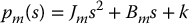

Figure 8.22 Idealized model to represent joint flexibility. The stiffness constant k represents the effective torsional stiffness of the harmonic gear.
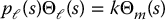
This system is represented by the block diagram of Figure 8.23. The output to be controlled is, of course, the load angle θℓ. The open-loop transfer function between U and Θℓ is given by

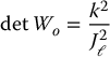
The open-loop characteristic polynomial pℓpm − k2 is

We can obtain some insigt! into the behavior of the system by first neglecting the damping coefficients Bℓ and Bm. In this case the open-loop characteristic polynomial would be

which has a double pole at the origin and a pair of complex conjugate poles on the jω-axis at s = ±jω where  . Note that the frequency of the imaginary poles increases with increasing joint stiffness k.

Figure 8.23 Block diagram for the system (8.59) and (8.60).
In practice the stiffness of the harmonic gear is large and the damping is small, which results in a difficult system to control. Assuming that the open-loop damping constants Bℓ and Bm are small, the open-loop poles of the system (8.59) and (8.60) will be in the left half plane near the poles of the undamped system.
Suppose we implement a PD compensator C(s) = KP + KDs. At this point the analysis depends on whether the position/velocity sensors are placed on the motor shaft or on the load shaft, that is, whether the PD compensator is a function of the motor variables or the load variables. If the motor variables are measured then the closed-loop system is given by the block diagram of Figure 8.24.

Figure 8.24 PD control with motor angle feedback.
If we measure the load angle θℓ instead, the system with PD control is represented by the block diagram of Figure 8.25. The corresponding root locus is shown in Figure 8.27.

Figure 8.25 PD control with load angle feedback.
Figure 8.26 shows the response of the system with motor feedback (left) and with link feedback (right!) using the PD controller KD(s + a).

Figure 8.26 Step response — PD control with motor angle feedback (left) and with link angle feedback (right!).
In order to perform a root locus we set KP + KDs = KD(s + a) with a = KP/KD. The root locus for the closed-loop systems in terms of KD is shown in Figure 8.27 for the case of a) motor angle feedback and b) load angle feedback.

Figure 8.27 Root loci for the flexible joint systems. a) represents motor-angle feedback and b) represents link-angle feedback.
In the case that the motor angle θm is used in the PD control, we see that the closed-loop system is stable for all values of the gain KD but that the presence of the open-loop zeros near the jω axis may result in undesirable oscillations. Also the poor relative stability means that disturbances and other unmodeled dynamics could render the system unstable.
In the case that the load angle θm is used in the PD control, we see that the closed-loop system is unstable for large KD. The critical value of KD, that is, the value of KD for which the system becomes unstable, can be found from the Routh–Hurwitz criterion. The best that one can do in this case is to limit the gain KD so that the closed-loop poles remain within the left half plane with a reasonable stability margin.
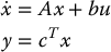
8.8 State Space Design
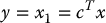
In this section we consider the application of state space methods for the control of the flexible joint system above.2 The previous analysis has shown that PD control is inadequate for robot control unless the joint flexibility is negligible or unless one is content with relatively slow response of the manipulator. Not only does the joint flexibility limit the magnitude of the gain for stability reasons, it also introduces ligt!ly damped poles into the closed-loop system that may result in oscillation in the transient response. We can write the system given by Equations (8.57) and (8.58) in state space by choosing state variables

In terms of these state variables the system given by Equations (8.57) and (8.58) becomes

which, in matrix form, can be written as
where
If we choose an output y(t), say the measured load angle θℓ(t), then we have an output equation
where

The relationship between the state space form given by Equations (8.68)–(8.71) and the transfer function (8.63) is found by taking Laplace transforms of Equations (8.68)–(8.70) with initial conditions set to zero. This yields
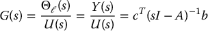
where I is the n × n identity matrix. The poles of G(s) are eigenvalues of the matrix A. For the system (8.68)–(8.71), the converse holds as well, that is, all of the eigenvalues of A are poles of G(s). This is always true if the state space system is defined using a minimal number of state variables.
8.8.1 State Feedback Control
Given a linear system in state space form, such as Equation (8.68), a linear state feedback control law is an input u of the form
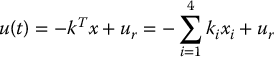
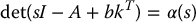
where ki are constant gains to be determined and ur is a reference input. In other words, the control is determined as a linear combination of the system states which, in this case, are the motor and load positions and velocities. Compare this to the previous PD/PID control, which was a function either of the motor position and velocity or of the load position and velocity, but not both. If we substitute the control law given by Equation (8.73) into Equation (8.68) we obtain
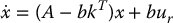
Thus, we see that the linear feedback control has the effect of changing the poles of the system from those determined by A to those determined by A − bkT.
In the previous PD designs the closed-loop pole locations were restricted to lie on the root locus plots shown in Figure 8.27. Since there are more free parameters in Equation (8.73) than in the PD controller, it may be possible to achieve a much larger range of closed-loop poles. This turns out to be the case if the system given by Equation (8.68) satisfies a property known as controllability.
Definition 8.1.
A linear system is said to be controllable if, for each initial state x(t0) and each final state x(tf), there is a control input t → u(t) that transfers the system from x(t0) at time t0 to x(tf) at time tf.
The above definition says, in essence, that if a system is controllable we can achieve any state whatsoever in finite time starting from an arbitrary initial state.
Let Wc be the n × n matrix3
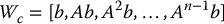
The matrix Wc is called the controllability matrix for the linear system defined by the pair (A, b). To check whether a system is controllable we have the following simple test.
Lemma 8.1
A linear system of the form (8.68) is controllable if and only if  .
.
The fundamental importance of controllability of a linear system is shown by the following
Theroem 8.1.
Let α(x) = sn + αn − 1sn − 1 + ⋅⋅⋅ + α1s + α0 be an arbitrary polynomial of degree n with real coefficients. Then there exists a state feedback control law of the form Equation (8.73) such that
if and only if the system (8.68) is controllable.
This fundamental result says that, for a controllable linear system, we may achieve arbitrary4 closed-loop poles using state feedback. Returning to the specific fourth-order system given by Equation (8.69), we see that the system is indeed controllable since

which is never zero since k > 0. Thus, we can achieve any desired set of closed-loop poles that we wish, which is much more than was possible using the previous PD compensator.
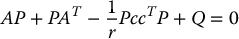
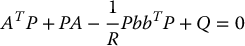
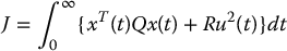
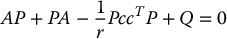
One way to design the feedback gains is through an optimization procedure. This takes us into the realm of optimal control theory. For example, we may choose as our goal the minimization of the performance criterion
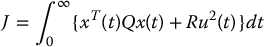
where Q is a given symmetric, positive definite matrix and R > 0.
Choosing a control law to minimize Equation (8.78) frees us from having to decide beforehand what the closed-loop poles should be as they are automatically dictated by the weigt!ing matrices Q and R in Equation (8.78). It is shown in optimal control texts that the optimum linear control law that minimizes Equation (8.78) is given as

where

and P is the unique symmetric, positive definite n × n matrix satisfying the so-called matrix algebraic Riccati equation

The control law (8.79) is referred to as a linear quadratic (LQ) optimal control, since the performance index is quadratic and the control system is linear.
8.8.2 Observers
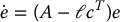
The above result that any set of closed-loop poles may be achieved for a controllable linear system is remarkable. However, to achieve it we have had to pay a price, namely, that the control law must be a function of all of the states. In order to build a compensator that requires only the measured output, in this case θℓ, we need to introduce the concept of an observer. An observer is a dynamical system (constructed in software) that attempts to estimate the full state x(t) using only the system model, Equations (8.68)–8.71), and the measured output y(t). A complete discussion of observers is beyond the scope of the present text. We give here only a brief introduction to the main idea of observers for linear systems.
Assuming that we know the parameters of the system (8.68) we could simulate the response of the system in software and recover the value of the state x(t) at time t from the simulation and we could use this simulated or estimated state, call it  , in place of the true state in Equation (8.79). However, since the true initial condition x(t0) for Equation (8.68) will generally be unknown, this idea is not feasible. However the idea of using the model of the system given by Equation (8.68) is a good starting point to construct a state estimator in software. Let us, therefore, consider an estimate
  of x(t) satisfying the system
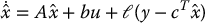
Equation (8.82) is called an observer for Equation (8.68) and represents a model of the system (8.68) with an additional term  . This additional term is a measure of the error between the output y(t) = cTx(t) of the plant and the estimate of the output,
  . Since we know the coefficient matrices in Equation (8.82) and can measure y directly, we can solve the above system for
  starting from any initial condition, and use this
  in place of the true state x in the feedback law (8.79). The additional term ℓ in Equation (8.82) is to be designed so that
  as t → ∞, that is, so that the estimated state converges to the true (unknown) state, independent of the initial condition x(t0). Let us see how this is done.
Define  as the estimation error. Combining Equations (8.68) and (8.82), since y = cTx, we see that the estimation error satisfies the system
From Equation (8.83) we see that the dynamics of the estimation error are determined by the eigenvalues of A − ℓcT. Since ℓ is a design quantity, we can attempt to choose it so that e(t) → 0 as t → ∞, in which case the estimate  converges to the true state x. In order to do this we obviously want to choose ℓ so that the eigenvalues of A − ℓcT are in the left half plane. This is similar to the pole assignment problem considered previously. In fact it is dual, in a mathematical sense, to the pole assignment problem. It turns out that the eigenvalues of A − ℓcT can be assigned arbitrarily if and only if the pair (A, c) satisfies the property known as observability. Observability is defined by the following:
Definition 8.2.
A linear system is observable if every initial state x(t0) can be exactly determined from measurements of the output y(t) and the input u(t) in a finite time interval t0 ⩽ t ⩽ tf.
Let Wo be the n × n matrix
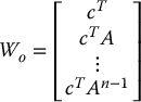
The matrix Wo in Equation (8.84) is called the observability matrix for the pair (cT, A). To check whether a system is observable we have the following
Lemma 8.2
The pair (cT, A) is observable if and only if  .
.
In the system given by Equations (8.68)–(8.71) above we have that
and hence the system is observable.
Note that the problem of finding the observer gains ℓ so that the matrix A − ℓcT has a prescribed set of eigenvalues is very similar to that of finding the state feedback gains k so that A − bkT has prescribed eigenvalues. In fact the two problems are  in a precise sense. Since the eigenvalues of A and AT are the same, we can define the following equivalences:

Using the above equivalences we can take the observer gains ℓ as

where P satisfies
for a given symmetric, positive definite matrix Q and R > 0. Now, if we use the estimated state  in place of the true state, we have the system (with r = 0)

It is easy to show from the above that the state x and estimation error e jointly satisfy the equation

and therefore the set of closed-loop poles of the system will consist of the union of the eigenvalues of A − ℓcT and the eigenvalues of A − bkT.
This result is known as the separation principle. As the name suggests, the separation principle allows us to separate the design of the state feedback control law (8.79) from the design of the state estimator (8.82). A typical procedure is to place the observer poles to the left of the desired pole locations of A − bkT. This results in rapid convergence of the estimated state to the true state, after which the response of the system is nearly the same as if the true state were being used in Equation (8.79). The reader can refer to Chapter 12 for a simulation of the observer-state feedback controller for the case of joint flexibility.
The result that the closed-loop poles of the system may be placed arbitrarily, under the assumption of controllability and observability, is a powerful theoretical result. There are always practical considerations to be taken into account, however. The most serious factor to be considered in observer design is noise in the measurement of the output. To place the poles of the observer very far to the left of the imaginary axis in the complex plane requires that the observer gains be large. Large gains can amplify noise in the output measurement and result in poor overall performance. Large gains in the state feedback control law (8.79) can result in saturation of the input, again resulting in poor performance. Also uncertainties in the system parameters, or nonlinearities such as a nonlinear spring characteristic and backlash, will reduce the achievable performance from the above design. Therefore, the above ideas are intended only to illustrate what may be possible by using more advanced concepts from control theory. In Chapter 9 we will develop more advanced, nonlinear control methods to control systems with uncertainties in the parameters.
8.9 Chapter Summary
This chapter is a basic introduction to robot control treating each joint of the manipulator as an independent single-input/single-output (SISO) system. In this approach one is primarily concerned with the actuator and drive-train dynamics.
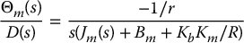
We first derived a reduced-order linear model for the dynamics of a permanent-magnet DC motor and showed that the transfer function from the motor voltage V(s) to the motor shaft angle Θm(s) can be expressed as
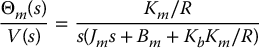
while the transfer function from a load disturbance D(s) to Θm(s) is
We then considered the set-point tracking problem using PD and PID compensators. A PD compensator is of the form

which results in a closed-loop system
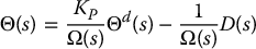
where
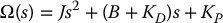
is the closed-loop characteristic polynomial whose roots determine the closed-loop poles and, hence, the performance of the system.
A PID compensator is of the form
The closed-loop system is now the third order system

where

We discussed methods to design the PD and PID gains for a desired transient and steady-state response. We then discussed the effects of saturation and flexibility on the performance of the system. Both of these effects limit the achievable performance of the closed-loop system.
Feedforward Control and Computed Torque
We next discussed the use of feedforward control as a method to track time varying reference trajectories such as the cubic polynomial trajectories that we derived in Chapter 7. A feedforward control scheme consists of adding a feedforward path from the reference signal to the control signal with transfer function F(s). We showed that choosing F(s) as the inverse of the forward plant allows tracking of arbitrary reference trajectories, provided that the forward plant is minimum phase.
We also introduced the notion of computed torque control, which is a feedforward disturbance cancellation method based on a computation of the nonlinear Euler-Lagrangian equations of motion. In the deal case the computed torque control, in effect, cancels the nonlinear dynamic coupling among the degrees of freedom of the manipulator and enhances the effectiveness of the linear feedback control methods in this chapter.
Joint Flexibility and State Space Methods
Next, we considered the effect of drive train dynamics in more detail. We derived a simple model for a single link system that included the joint elasticity and showed the limitations of PD control for this case. We then introduced state space control methods, which are much more powerful than the simple PD and PID control methods.
We introduced the fundamental notions of controllability and observability and showed that, if the state space model is both controllable and observable, we could design a linear control law to achieve any set of desired closed-loop poles. Specifically, given the linear system
then the state feedback control law  where
where  is the estimate of the state x computed from a linear observer

results in the closed-loop system (in terms of the state x and estimation error  )
)
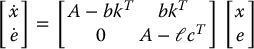
The set of closed-loop poles of the system will therefore consist of the union of the eigenvalues of A − ℓcT and the eigenvalues of A − bkT, a result known as the separation principle.
We also introduced the notion of linear quadratic optimal control and showed that the control

where

and P is the (unique) symmetric, positive definite n × n matrix satisfying the so-called matrix algebraic Riccati equation
not only stabilizes the system but minimizes the quadratic performance measure
Using the duality between control and observation, we showed that the observer gain ℓ could likewise be chosen as

where P satisfies
Problems
- Using block diagram reduction techniques derive the transfer functions given by Equations (8.11) and (8.12).
- Derive the transfer functions for the reduced-order model given by Equations (8.13) and (8.14).
- Derive Equations (8.35) and (8.36).
- Verify the computation of the closed-loop compensators in Table 8.1.
- Verify the expression given by Equation (8.37) for the tracking error for the system in Figure 8.11. State the Final Value Theorem and use it to show that the steady-state error ess is indeed given by Equation (8.40).
- Derive Equations (8.45) and (8.46).
- Derive the inequality (8.47) using the Routh–Hurwitz criterion.
- For the system of Figure 8.14 investigate the effect of saturation with various values of the PID gains and disturbance magnitude.
- Verify Equation (8.49).
- Verify Equation (8.52).
- Derive Equations (8.63), (8.64), and (8.65).
- Given the state space model defined by Equation (8.68) show that the transfer function
is identical to Equation (8.63).

- Search the control literature (for example, [71]) and find two or more algorithms for the pole assignment problem for linear systems.
- Derive Equations (8.77) and (8.85).
- Search the control literature to find out what is meant by integrator windup. Find out what is meant by anti-windup(or anti-reset windup). Simulate a PID control with anti-reset windup for the system of Figure 8.14. Compare the response with and without anti-reset windup.
- Include the dynamics of a permanent magnet DC motor for the system given by Equations (8.57) and (8.58). What can you say now about controllability and observability of the system?
- Choose appropriate state variables and write the system Equations (8.9) and (8.10) in state space form. What is the dimension of the state space?
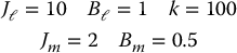
- Suppose in the flexible joint system represented by Equations (8.57) and (8.58) the following parameters are given
- Sketch the open-loop poles of the transfer functions given by Equation (8.63).
- Apply a PD compensator to the system (8.63). Sketch the root locus for the system. Choose a reasonable location for the compensator zero. Using the Routh criterion, find the value of the compensator gain when the root locus crosses the imaginary axis.
-
One of the problems encountered in space applications of robots is the fact that the base of the robot cannot be anchored, that is, cannot be fixed in an inertial coordinate frame. Consider the idealized situation shown in Figure 8.28, consisting of an inertia J1 connected to the rotor of a motor whose stator is connected to an inertia J2.
For example, J1 could represent the space shuttle robot arm and J2 the inertia of the shuttle itself. The simplified equations of motion are thus

Write this system in state space form and show that it is uncontrollable. Discuss the implications of this and suggest possible solutions.
-
Given the linear second-order system
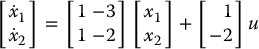
find a linear state feedback control u = k1x1 + k2x2 so that the closed-loop system has poles at s = −2, 2.
- Consider the block diagram of Figure 8.17. Suppose that G(s) = 1/(2s2 + s) and suppose that it is desired to track a reference signal θd(t) = sin (t) + cos (2t). If we further specify that the closed-loop system should have a natural frequency less than 10 radians with a damping ratio greater than 0.707, compute an appropriate compensator C(s) and feedforward transfer function F(s).

Figure 8.28 Coupled inertias in free space.
Notes and References
Although we treated only the dynamics of permanent magnet DC motors, the use of AC motors is increasing in robotics and other types of motion control applications. AC motors do not require commutators and brushes and so are inherently more maintenance free and reliable. However, they are more difficult to control and require more sophisticated power electronics. With recent advances in power electronics together with their decreasing cost, AC motors may soon replace DC motors as the dominant actuation method for robot manipulators. A reference that treats different types of motors is [57].
A good background text on linear control systems is [84]. For a text that treats PID control in depth, consult [8].
The pole assignment theorem is due to Wonham [185]. The notion of controllability and observability, introduced by Kalman in [72], arises in several fundamental ways in addition to those discussed here. The interested reader should consult various references on the Kalman filter, which is a linear state estimator for systems whose output measurements are corrupted by (stochastic, white) noise. The linear observer that we discuss here was introduced by Luenberger [103] and is often referred to as the deterministic Kalman filter. Luenberger’s main contribution in [103] was in the so-called reduced-order observer, which allows one to reduce the dimension of the observer.
Linear quadratic optimal control, in its present form, was introduced by Kalman in [72], where the importance of the Riccati equation was emphasized. The field of linear control theory is broad and there are many other techniques available to design state-feedback and output-feedback control laws in addition to the basic optimal control approach considered here. More recent control system design methods include the H∞ approach [36] as well as approaches based on fuzzy logic [133] and neural networks [94] and [52].
The problem of drive-train dynamics in robotics was first pointed out by Good and Sweet, who studied the dynamics of the General Electric P-50 robot (see [172]). For this and other early robots the limiting factors to performance were current limiters that limited how much current could be drawn by the motors and elasticity in the joints due to gear flexibility. Both effects limit the maximum attainable safe speed at which the robot can operate. This work stimulated considerable research into the control of robots with input constraints (see [169]) and the control of robots with flexible joints (see [165]).
Finally, virtually all robot control systems today are implemented digitally. A treatment of digital control requires consideration of issues of sampling, quantization, resolution, as well as computer architecture, real-time programming and other issues that are not considered in this chapter. The interested reader should consult, for example, [48] for these latter subjects.
Notes
- 1 MKS units are based on the meter, kilogram, and second.
- 2 This section assumes more knowledge of control theory than previous sections.
- 3 For a system with m control inputs Wc will have dimension n × nm
- 4 Since the coefficients of the polynomial a(s) are real, the only restriction on the pole locations is that they occur in complex conjugate pairs.