CHAPTER 6
DYNAMICS
This chapter deals with the dynamics of robot manipulators. Whereas the kinematic equations describe the motion of the robot without consideration of the forces and torques producing the motion, the dynamic equations explicitly describe the relationship between force and motion. The equations of motion are important to consider in the design of robots, in simulation and animation of robot motion, and in the design of control algorithms. We introduce the so-called Euler–Lagrange equations, which describe the evolution of a mechanical system subject to holonomic constraints (this term is defined later on). To motivate the Euler–Lagrange approach we begin with a simple derivation of these equations from Newton’s second law for a one-degree-of-freedom system. We then derive the Euler–Lagrange equations from the principle of virtual work in the general case.
In order to determine the Euler-Lagrange equations in a specific situation, one has to form the Lagrangian of the system, which is the difference between the kinetic energy and the potential energy; we show how to do this in several commonly encountered situations. We then derive the dynamic equations of several example robotic manipulators, including a two-link Cartesian robot, a two-link planar robot, and a two-link robot with remotely driven joints.
We also discuss several important properties of the Euler–Lagrange equations that can be exploited to design and analyze feedback control algorithms. Among these are explicit bounds on the inertia matrix, linearity in the inertia parameters, and the skew symmetry and passivity properties.
This chapter is concluded with a derivation of an alternate formulation of the dynamical equations of a robot, known as the Newton–Euler formulation, which is a recursive formulation of the dynamic equations that is often used for numerical calculation and simulation.
6.1 The Euler–Lagrange Equations
In this section we present a general set of differential equations that describe the time evolution of mechanical systems subjected to holonomic constraints when the constraint forces satisfy the principle of virtual work. These are called the Euler-Lagrange equations of motion. Note that there are at least two distinct ways of deriving these equations. The method presented here is based on the method of virtual work, but it is also possible to derive the same equations using Hamilton’s principle of least action.
6.1.1 Motivation
To motivate the subsequent discussion, we show first how the Euler–Lagrange equations can be derived from Newton’s second law for the one-degree-of-freedom system shown in Figure 6.1.
By Newton’s second law, the equation of motion of the particle is
Notice that the left-hand side of Equation (6.1) can be written as
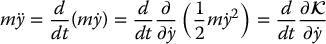
where  is the kinetic energy. We use the partial derivative notation in the above expression to be consistent with systems considered later when the kinetic energy will be a function of several variables. Likewise we can express the gravitational force in Equation (6.1) as
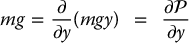
where  is the potential energy due to gravity. If we define
and note that
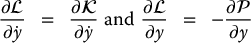
then we can write Equation (6.1) as
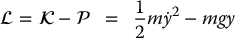
The function  , which is the difference of the kinetic and potential energy, is called the Lagrangian of the system, and Equation (6.5) is called the Euler–Lagrange equation.

Figure 6.1 A particle of constant mass m constrained to move vertically constitutes a one-degree-of-freedom system. The gravitational force mg acts downward and an external force f acts upward.
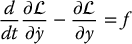
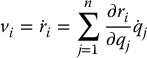
The general procedure that we discuss below is, of course, the reverse of the above; namely, one first writes the kinetic and potential energies of a system in terms of a set of so-called generalized coordinates (q1, …, qn), where n is the number of degrees of freedom of the system, and then computes the equations of motion of the n-DOF system according to
where τk is the (generalized) force associated with qk. In the above single DOF example, the variable y serves as the generalized coordinate. Application of the Euler–Lagrange equations leads to a set of coupled second-order ordinary differential equations and provides a formulation of the dynamic equations of motion for serial-link robots equivalent to those derived using Newton’s second law. However, as we shall see, the Lagrangian approach is advantageous for complex systems such as multi-link robots.
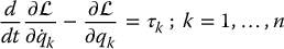
Example 6.1. (Single-Link Manipulator).
Consider the single-link robot arm shown in Figure 6.2, consisting of a rigid link coupled through a gear train to a DC motor. Let θℓ and θm denote the angles of the link and motor shaft, respectively. Then, θm = rθℓ where r: 1 is the gear ratio. The algebraic relation between the link and motor shaft angles means that the system has only one degree of freedom and we can therefore use as generalized coordinate either θm or θℓ.
If we choose as generalized coordinate q = θℓ, the kinetic energy of the system is given by
where Jm, Jℓ are the rotational inertias of the motor and link, respectively. The potential energy is given as
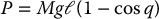
where M is the total mass of the link and ℓ is the distance from the joint axis to the link center of mass. Defining I = r2Jm + Jℓ, the Lagrangian  is given by
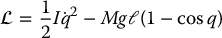
Substituting this expression into the Equation (6.6) with n = 1 and generalized coordinate θℓ yields the equation of motion
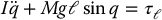
The generalized force τℓ represents those external forces and torques that are not derivable from a potential function. For this example, τℓ consists of the input motor torque u = rτm, reflected to the link, and (nonconservative) damping torques  and
and  . Reflecting the motor damping to the link yields

where B = rBm + Bℓ. Therefore, the complete expression for the dynamics of this system is

Example 6.2. (Single-Link Manipulator with Elastic Joint).
Next, consider a single-link manipulator including the transmission flexibility as shown in Figure 6.3.
In this case the motor angle q1 = θℓ and the link angle q2 = θm are independent variables and so the system possesses two degrees of freedom. Thus, two generalized coordinates are required to specify the configuration of the system.
The kinetic energy of this system is
The potential energy includes the spring potential energy in addition to the gravitational potential energy,
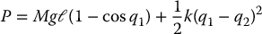
Forming the Lagrangian  and ignoring damping for simplicity, the equations of motion are found from the Euler-Lagrange equations as
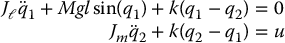
The details are left as an exercise (Problem 6–1).

Figure 6.2 Single-link robot. The motor shaft is coupled to the axis of rotation of the link through a gear train which amplifies the motor torque and reduces the motor speed.

Figure 6.3 Single-link, flexible-joint robot. The joint elasticity arises from flexibility in the shaft or gears.
6.1.2 Holonomic Constraints and Virtual Work
Now, consider a system of k particles with corresponding position vectors r1, …, rk as shown in Figure 6.4.

Figure 6.4 An unconstrained system of k particles has 3k degrees of freedom. If the particles are constrained, the number of degrees of freedom is reduced.
If these particles are free to move about without any restrictions, then it is quite an easy matter to describe their motion, by noting that the mass times acceleration of each particle equals the external force applied to it. However, if the motion of the particles is constrained in some fashion, then one must take into account not only the externally applied forces, but also the so-called constraint forces, that is, the forces needed to make the constraints hold. As a simple illustration of this, suppose the system consists of two particles joined by a massless rigid wire of length ℓ. Then the two coordinates r1 and r2 must satisfy the constraint

If one applies some external forces to each particle, then the particles experience not only these external forces but also the force exerted by the wire, which is along the direction r2 − r1 and of appropriate magnitude. Therefore, in order to analyze the motion of the two particles, we could follow one of two options. We could compute, under each set of external forces, what the corresponding constraint force must be in order that the equation above continues to hold. Alternatively, we can search for a method of analysis that does not require us to know the constraint force. Clearly, the second alternative is preferable, since it is generally quite an involved task to compute the constraint forces. This section is aimed at achieving this latter objective.
First, it is necessary to introduce some terminology. A constraint on the k coordinates r1, …, rk is called holonomic if it is an equality constraint of the form

The constraint given in Equation (6.15) imposed by connecting two particles by a massless rigid wire is an example of a holonomic constraint. By differentiating Equation (6.16) we have an expression of the form
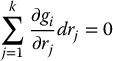
A constraint of the form
is called nonholonomic if it cannot be integrated to an equality constraint of the form (6.16). It is interesting to note that, while the method of deriving the equations of motion using the principle of virtual work remains valid for nonholonomic systems, methods based on variational principles, such as Hamilton’s principle, can no longer be applied to derive the equations of motion. We will discuss systems subject to nonholonomic constraints in Chapter 14.
If a system is subjected to ℓ holonomic constraints, then one can think in terms of the constrained system having ℓ fewer degrees of freedom than the unconstrained system. In this case, it may be possible to express the coordinates of the k particles in terms of n generalized coordinates q1, …, qn. In other words, we assume that the coordinates of the various particles, subjected to the set of constraints given by Equation (6.16), can be expressed in the form

where q1, …, qn are all independent. In fact, the idea of generalized coordinates can be used even when there are infinitely many particles. For example, a physical rigid object such as a bar contains an infinity of particles; but since the distance between each pair of particles is fixed throughout the motion of the bar, six coordinates are sufficient to specify completely the coordinates of any particle in the bar. In particular, one could use three position coordinates to specify the location of the center of mass of the bar, and three Euler angles to specify the orientation of the body. Typically, generalized coordinates are positions, angles, etc. In fact, in Chapter 3 we chose to denote the joint variables by the symbols q1, …, qn precisely because these joint variables form a set of generalized coordinates for an n-link robot manipulator.
One can now speak of virtual displacements, which are any set of infinitesimal displacements, δr1, …, δrk, that are consistent with the constraints. For example, consider once again the constraint (6.15) and suppose r1, r2 are perturbed to r1 + δr1, r2 + δr2, respectively. Then, in order that the perturbed coordinates continue to satisfy the constraint, the length of the bar must not change and so we must have

Now, let us expand the above product and take advantage of the fact that the original coordinates r1, r2 satisfy the constraint given by Equation (6.15). If we neglect quadratic terms in δr1, δr2 we obtain after some algebra (Problem 6–2)
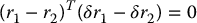
Thus, any infinitesimal perturbations in the positions of the two particles must satisfy the above equation in order that the perturbed positions continue to satisfy the constraint Equation (6.15). Any pair of infinitesimal vectors δr1, δr2 that satisfy Equation (6.21) constitutes a set of virtual displacements for this problem. Figure 6.5 shows some representative virtual displacements for a rigid bar.

Figure 6.5 Examples of virtual displacements for a rigid bar. These infinitesimal motions do not change the distance between the endpoints and are thus compatible with the assumption that the bar is rigid.
Now, the reason for using generalized coordinates is to avoid dealing with complicated relationships such as Equation (6.21) above. If Equation (6.19) holds, then one can see that the set of all virtual displacements is precisely
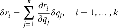
where the virtual displacements δq1, …, δqn of the generalized coordinates are unconstrained (that is what makes them generalized coordinates).
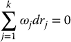
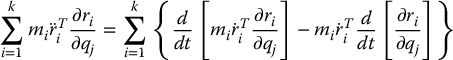
Next, we begin a discussion of constrained systems in equilibrium. Suppose each particle is in equilibrium. Then the net force on each particle is zero, which in turn implies that the work done by each set of virtual displacements is zero. Hence, the sum of the work done by any set of virtual displacements is also zero; that is,
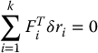
where Fi is the total force on particle i. As mentioned earlier, the force Fi is the sum of two quantities, namely (i) the externally applied force fi, and (ii) the constraint force fai. Now, suppose that the total work done by the constraint forces corresponding to any set of virtual displacements is zero, that is,
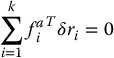
This will be true whenever the constraint force between a pair of particles is directed along the radial vector connecting the two particles (see the discussion in the next paragraph). Substituting Equation (6.24) into Equation (6.23) results in
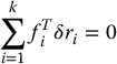
The beauty of this equation is that it does not involve the unknown constraint forces, but only the known external forces. This equation expresses the principle of virtual work, which can be stated in words as: The work done by external forces corresponding to any set of virtual displacements is zero.
Note that the principle is not universally applicable; it requires that Equation (6.24) hold, that is, that the constraint forces do no work. Thus, if the principle of virtual work applies, one can analyze the dynamics of a system without having to evaluate the constraint forces.
It is easy to verify that the principle of virtual work applies whenever the constraint force between a pair of particles acts along the vector connecting the position coordinates of the two particles. In particular, when the constraints are of the form (6.15), the principle applies. To see this, consider once again a single constraint of the form (6.15). In this case, the constraint force, if any, must be exerted by the rigid massless wire, and therefore must be directed along the radial vector connecting the two particles. In other words, the force exerted on the first particle by the wire must be of the form
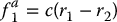
for some constant c (which could change as the particles move about). By the law of action and reaction, the force exerted on the second particle by the wire must be just the negative of the above, that is,
Now, the work done by the constraint forces corresponding to a set of virtual displacements is

But, Equation (6.21) shows that the above expression must be zero for any set of virtual displacements. The same reasoning can be applied if the system consists of several particles that are pairwise connected by rigid massless wires of fixed lengths, in which case the system is subjected to several constraints of the form (6.15). Now, the requirement that the motion of a body be rigid can be equivalently expressed as the requirement that the distance between any pair of points on the body remain constant as the body moves, that is, as an infinity of constraints of the form (6.15). Thus, the principle of virtual work applies whenever rigidity is the only constraint on the motion. There are indeed situations when this principle does not apply, such as in the presence of magnetic fields. However, in all situations encountered in this book, we can safely assume that the principle of virtual work is valid.
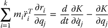
6.1.3 D’Alembert’s Principle
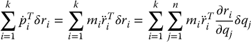
In Equation (6.25), the virtual displacements δri are not independent, so we cannot conclude from this equation that each coefficient Fi individually equals zero. In order to apply such reasoning, we must transform to generalized coordinates. Before doing this, we consider systems that are not necessarily in equilibrium. For such systems, D’Alembert’s principle states that, if one introduces a fictitious additional force  on each particle, where pi is the momentum of particle i, then each particle will be in equilibrium. Thus, if one modifies Equation (6.23) by replacing Fi by
  , then the resulting equation is valid for arbitrary systems. One can then remove the constraint forces as before using the principle of virtual work. This results in the equation
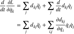
The above equation does not mean that each coefficient of δri is zero since the virtual constraints δri are not independent. The remainder of this derivation is aimed at expressing the above equation in terms of the generalized coordinates, which are independent. For this purpose, we express each δri in terms of the corresponding virtual displacements of generalized coordinates, as is done in Equation (6.22). Then, the virtual work done by the forces fi is given by
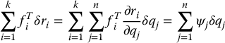
where
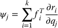
is called the jth generalized force. Note that ψj need not have dimensions of force, just as qj need not have dimensions of length; however, ψjδqj must always have dimensions of work.
Now, let us study the second summation in Equation (6.29). Since  , it follows that
Next, using the product rule of differentiation, we have
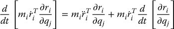
Rearranging the above and summing over all i = 1, …, n yields
Now, differentiating Equation (6.19) using the chain rule gives
Observe from the above equation that

Next,
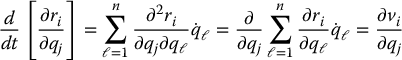
where the last equality follows from Equation (6.35). Substituting from Equation (6.36) and Equation (6.37) into Equation (6.34) and noting that  gives
gives
If we define the kinetic energy K to be the quantity
then Equation (6.38) can be compactly expressed as
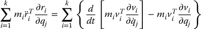
Now, substituting from Equation (6.40) into Equation (6.32) shows that the second summation in Equation (6.29) is
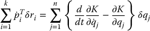
Finally, combining Equations (6.29), (6.30), and (6.41) gives
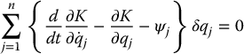
Now, since the virtual displacements δqj are independent, we can conclude that each coefficient in Equation (6.42) is zero, that is,

If the generalized force ψj is the sum of an externally applied generalized force and another one due to a potential field, then a further modification is possible. Suppose there exist functions τj and a potential energy function P(q) such that
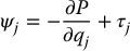
Then Equation (6.43) can be written in the form
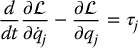
where  is the Lagrangian and we have recovered the Euler–Lagrange equations of motion as in Equation (6.6).
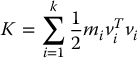
6.2 Kinetic and Potential Energy
In the previous section, we showed that the Euler–Lagrange equations can be used to derive the dynamical equations in a straightforward manner, provided one is able to express the kinetic and potential energies of the system in terms of a set of generalized coordinates. In order for this result to be useful in a practical context, it is important that one be able to compute these terms readily for an n-link robotic manipulator. In this section we derive formulas for the kinetic energy and potential energy of a robot with rigid links using the Denavit–Hartenberg joint variables as generalized coordinates.
To begin we note that the kinetic energy of a rigid object is the sum of two terms, the translational kinetic energy obtained by concentrating the entire mass of the object at the center of mass, and the rotational kinetic energy of the body about the center of mass. Referring to Figure 6.6 we attach a coordinate frame at the center of mass (called the body-attached frame) as shown.

Figure 6.6 A general rigid body has six degrees of freedom. The kinetic energy consists of kinetic energy of rotation and kinetic energy of translation.
The kinetic energy of the rigid body is then given as
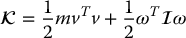
where m is the total mass of the object, v and ω are the linear and angular velocity vectors, respectively, and  is a symmetric 3 × 3 matrix called the inertia tensor.
6.2.1 The Inertia Tensor
It is understood that the above linear and angular velocity vectors, v and ω, respectively, are expressed in the inertial frame. In this case, we know that ω is found from the skew-symmetric matrix

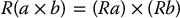
where R is the orientation transformation from the body-attached frame and the inertial frame. It is therefore necessary to express the inertia tensor,  , also in the inertial frame in order to compute the triple product
  . The inertia tensor relative to the inertial reference frame will depend on the configuration of the object. If we denote as I the inertia tensor expressed instead in the body-attached frame, then the two matrices are related via a similarity transformation according to

This is an important observation because the inertia matrix expressed in the body-attached frame is a constant matrix independent of the motion of the object and easily computed.
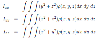
We next show how to compute this matrix explicitly. Let the mass density of the object be represented as a function of position, ρ(x, y, z). Then the inertia tensor in the body attached frame is computed as
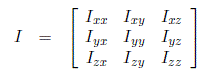
where
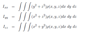
and
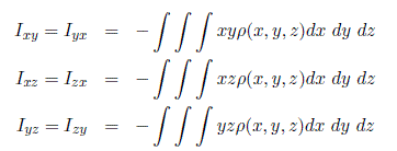
The integrals in the above expression are computed over the region of space occupied by the rigid body. The diagonal elements of the inertia tensor, Ixx, Iyy, Izz, are called the principal moments of inertia about the x, y, and z-axes, respectively. The off-diagonal terms Ixy, Ixz, etc., are called the cross products of inertia. If the mass distribution of the body is symmetric with respect to the body-attached frame, then the cross products of inertia are identically zero.
Example 6.3. (Uniform Rectangular Solid).
Consider the rectangular solid of length a width b and height c shown in Figure 6.7 and suppose that the density is constant, ρ(x, y, z) = ρ. If the body frame is attached at the geometric center of the object, then by symmetry, the cross products of inertia are all zero and it is a simple exercise to compute
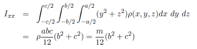
since ρabc = m, the total mass. Likewise, a similar calculation shows that
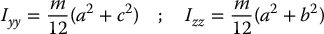

Figure 6.7 A rectangular solid with uniform mass density and coordinate frame attached at the geometric center of the solid.
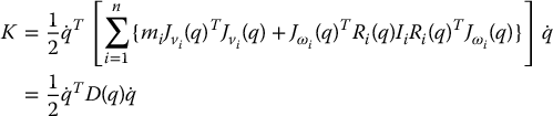
6.2.2 Kinetic Energy for an n-Link Robot
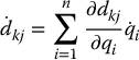
Now, consider a manipulator with n links. We have seen in Chapter 4 that the linear and angular velocities of any point on any link can be expressed in terms of the Jacobian matrix and the derivatives of the joint variables. Since, in our case, the joint variables are indeed generalized coordinates, it follows that, for appropriate Jacobian matrices  and
and  , of dimension 3 × n, we have

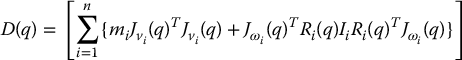
Now, suppose the mass of link i is mi and that the inertia matrix of link i, evaluated around a coordinate frame parallel to frame i but whose origin is at the center of mass, equals Ii. Then from Equations (6.46) and (6.50) it follows that the overall kinetic energy of the manipulator equals
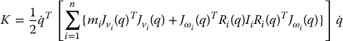
where

is an n × n configuration dependent matrix called the inertia matrix. In Section 6.4 we will compute this matrix for several commonly occurring manipulator configurations. The inertia matrix is symmetric and positive definite for any manipulator. Symmetry of D(q) is easily seen from Equation (6.53). Positive definiteness can be inferred from the fact that the kinetic energy is always nonnegative and is zero if and only if all of the joint velocities are zero. The formal proof is left as an exercise (Problem 6–6).
6.2.3 Potential Energy for an n-Link Robot
Now, consider the potential energy term. In the case of rigid dynamics, the only source of potential energy is gravity. The potential energy of the ith link can be computed by assuming that the mass of the entire object is concentrated at its center of mass and is given by

where g is the vector giving the direction of gravity in the inertial frame and the vector rci gives the coordinates of the center of mass of link i. The total potential energy of the n-link robot is therefore

In the case that the robot contains elasticity, for example if the joints are flexible, then the potential energy will include terms containing the energy stored in the elastic elements. Note that the potential energy is a function only of the generalized coordinates and not their derivatives.
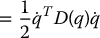
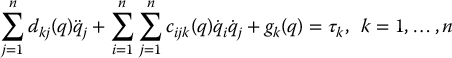
6.3 Equations of Motion
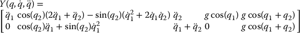
In this section we specialize the Euler–Lagrange equations derived in Section 6.1 to the case when two conditions hold. First, the kinetic energy is a quadratic function of the vector  of the form

where di, j are the entries of the n × n inertia matrix D(q), which is symmetric and positive definite for each  , and second, the potential energy P = P(q) is independent of
  . We have already remarked that robotic manipulators satisfy these conditions.
The Euler–Lagrange equations for such a system can be derived as follows. Using Equation (6.56) we can write the Lagrangian as
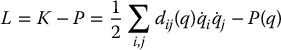
The partial derivatives of the Lagrangian with respect to the kth joint velocity is given by
and therefore
Similarly the partial derivative of the Lagrangian with respect to the kth joint position is given by
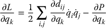
Thus, for each k = 1, …, n, the Euler–Lagrange equations can be written
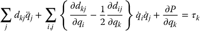
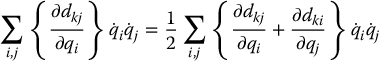
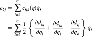
By interchanging the order of summation and taking advantage of symmetry, one can show (Problem 6–7) that
Hence
where we define
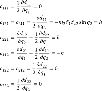
The terms cijk in Equation (6.63) are known as Christoffel symbols (of the first kind). Note that, for a fixed k, we have cijk = cjik, which reduces the effort involved in computing these symbols by a factor of about one half. Finally, if we define

then we can write the Euler–Lagrange equations as

In the above equations, there are three types of terms. The first type involves the second derivative of the generalized coordinates. The second type involves quadratic terms in the first derivatives of q, where the coefficients may depend on q. These latter terms are further classified into those involving a product of the type  and those involving a product of the type
  where i ≠ j. Terms of the type
  are called centrifugal, while terms of the type
  are called Coriolis terms. The third type of terms are those involving only q but not its derivatives. This third type arises from differentiating the potential energy. It is common to write Equation (6.65) in matrix form as

where the (k, j)th element of the matrix  is defined as
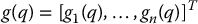
and the gravity vector g(q) is given by
In summary, the development in this section is very general and applies to any mechanical system whose kinetic energy is of the form (6.56) and whose potential energy is independent of  . In the next section we apply this discussion to study specific robot configurations.
6.4 Some Common Configurations
In this section we apply the above method of analysis to several manipulator configurations and derive the corresponding equations of motion. The configurations are progressively more complex, beginning with a two-link Cartesian manipulator and ending with a five-bar linkage mechanism that has a particularly simple inertia matrix.
Two-Link Cartesian Manipulator
Consider the manipulator shown in Figure 6.8 consisting of two links and two prismatic joints. Denote the masses of the two links by m1 and m2, respectively, and denote the displacement of the two prismatic joints by q1 and q2, respectively. It is easy to see, as mentioned in Section 6.1, that these two quantities serve as generalized coordinates for the manipulator. Since the generalized coordinates have dimensions of distance, the corresponding generalized forces have units of force. In fact, they are just the forces applied at each joint. Let us denote these by fi, i = 1, 2.

Figure 6.8 Two-link planar Cartesian robot. The orthogonal joint axes and linear joint motion of the Cartesian robot result in simple kinematics and dynamics.
Since we are using the joint variables as the generalized coordinates, we know that the kinetic energy is of the form (6.56) and that the potential energy is only a function of q1 and q2. Hence, we can use the formulas in Section 6.3 to obtain the dynamical equations. Also, since both joints are prismatic, the angular velocity Jacobian is zero and the kinetic energy of each link consists solely of the translational term.
It follows that the velocity of the center of mass of link 1 is given by

where

Similarly,

where
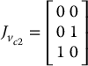
Hence, the kinetic energy is given by
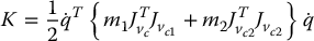
Comparing with Equation (6.56), we see that the inertia matrix D is given simply by
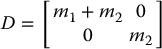
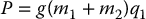
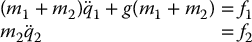
Next, the potential energy of link 1 is m1gq1, while that of link 2 is m2gq1, where g is the acceleration due to gravity. Hence, the overall potential energy is
Now, we are ready to write down the equations of motion. Since the inertia matrix is constant, all Christoffel symbols are zero. Furthermore, the components gk of the gravity vector are given by
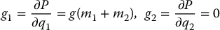
Substituting into Equation (6.65) gives the dynamical equations as
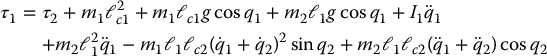
Planar Elbow Manipulator
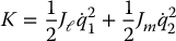
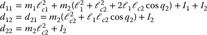
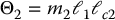
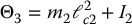
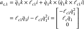
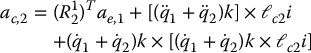
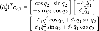
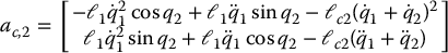
Now, consider the planar manipulator with two revolute joints shown in Figure 6.9. Let us fix notation as follows: For i = 1, 2, qi denotes the joint angle, which also serves as a generalized coordinate; mi denotes the mass of link i; ℓi denotes the length of link i; ℓci denotes the distance from the previous joint to the center of mass of link i; and Ii denotes the moment of inertia of link i about an axis coming out of the page, passing through the center of mass of link i.

Figure 6.9 Two-link revolute joint arm. The rotational joint motion introduces dynamic coupling between the joints.
We will use the Denavit–Hartenberg joint variables as generalized coordinates, which will allow us to make effective use of the Jacobian expressions in Chapter 4 in computing the kinetic energy. First,

where,
Similarly,

where
Hence, the translational part of the kinetic energy is

Next, we consider the angular velocity terms. Because of the particularly simple nature of this manipulator, many of the potential difficulties do not arise. First, it is clear that

when expressed in the base inertial frame. Moreover, since ωi is aligned with the z-axes of each joint coordinate frame, the rotational kinetic energy reduces simply to  , where Ii is the moment of inertia about an axis through the center of mass of link i parallel to the zi-axis. Hence, the rotational kinetic energy of the overall system in terms of the generalized coordinates is
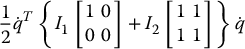
Now, we are ready to form the inertia matrix D(q). For this purpose, we merely have to add the two matrices in Equation (6.82) and Equation (6.84), respectively. Thus
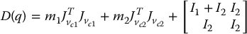
Carrying out the above multiplications and using the standard trigonometric identities cos 2θ + sin 2θ = 1, cos αcos β + sin αsin β = cos (α − β) leads to
Now, we can compute the Christoffel symbols using Equation (6.63). This gives
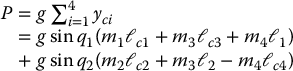
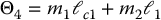
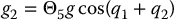
Next, the potential energy of the manipulator is just the sum of those of the two links. For each link, the potential energy is just its mass multiplied by the gravitational acceleration and the height of its center of mass. Thus
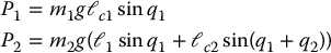
and so the total potential energy is

Therefore, the functions gk defined in Equation (6.64) become

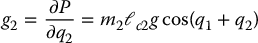
Finally, we can write down the dynamical equations of the system as in Equation (6.65). Substituting for the various quantities in this equation and omitting zero terms leads to
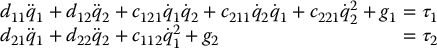
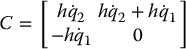
In this case, the matrix  is given as
Planar Elbow Manipulator with Remotely Driven Link
Now, we illustrate the use of Lagrangian equations in a situation where the generalized coordinates are not the joint variables defined in earlier chapters. Consider again the planar elbow manipulator, but suppose now that both joints are driven by motors mounted at the base. The first joint is turned directly by one of the motors, while the other is turned via a gearing mechanism or a timing belt (see Figure 6.10).

Figure 6.10 Two-link revolute joint arm with remotely driven link. Because of the remote drive the motor shaft angles are not proportional to the joint angles.
In this case, one should choose the generalized coordinates as shown in Figure 6.11, because the angle p2 is determined by driving motor number 2, and is not affected by the angle p1. We will derive the dynamical equations for this configuration and show that some simplifications will result.

Figure 6.11 Generalized coordinates for the robot of Figure 6.10.
Since p1 and p2 are not the joint angles used earlier, we cannot use the velocity Jacobians derived in Chapter 4 in order to find the kinetic energy of each link. Instead, we have to carry out the analysis directly. It is easy to see that

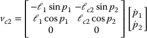
Hence, the kinetic energy of the manipulator equals
where
Computing the Christoffel symbols as in Equation (6.63) gives
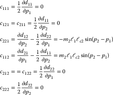
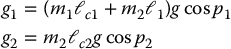
Next, the potential energy of the manipulator, in terms of p1 and p2, equals

Hence, the gravitational generalized forces are
Finally, the equations of motion are

Comparing Equation (6.99) and Equation (6.90), we see that by driving the second joint remotely from the base we have eliminated the Coriolis forces, but we still have the centrifugal forces coupling the two joints.
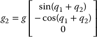
Five-Bar Linkage
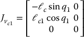
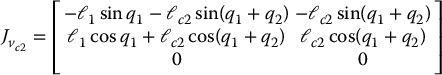
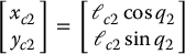
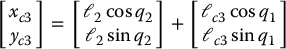
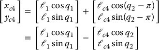
Now, consider the manipulator shown in Figure 6.12. We will show that, if the parameters of the manipulator satisfy a simple relationship, then the equations of the manipulator are decoupled, so that each quantity q1 and q2 can be controlled independently of the other. The mechanism in Figure 6.12 is called a five-bar linkage. Clearly, there are only four bars in the figure, but in the theory of mechanisms it is a convention to count the ground as an additional linkage, which explains the terminology. It is assumed that the lengths of links 1 and 3 are the same, and that the two lengths marked ℓ2 are the same; in this way the closed path in the figure is in fact a parallelogram, which greatly simplifies the computations. Notice, however, that the quantities ℓc1 and ℓc3 need not be equal. For example, even though links 1 and 3 have the same length, they need not have the same mass distribution. It is clear from the figure that, even though there are four links being moved, there are in fact only two degrees of freedom, identified as q1 and q2. Thus, in contrast to the earlier mechanisms studied in this book, this one is a closed kinematic chain (though of a particularly simple kind). As a result, we cannot use the earlier results on Jacobian matrices, and instead have to start from scratch. As a first step we write down the coordinates of the centers of mass of the various links as a function of the generalized coordinates. This gives

Figure 6.12 Five-bar linkage.

Next, with the aid of these expressions, we can write down the velocities of the various centers of mass as a function of  and
and  . For convenience we drop the third row of each of the following Jacobian matrices as it is always zero. The result is
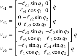
Let us define the velocity Jacobians  , i ∈ {1, …, 4} in the obvious fashion, that is, as the four matrices appearing in the above equations. Next, it is clear that the angular velocities of the four links are simply given by

Thus, the inertia matrix is given by

If we now substitute from Equation (6.104) into the above equation and use the standard trigonometric identities, we are left with
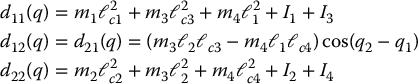
Now, we note from the above expressions that if
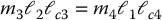
then d12 and d21 are zero, that is, the inertia matrix is diagonal and constant. As a consequence the dynamical equations will contain neither Coriolis nor centrifugal terms.
Turning now to the potential energy, we have that
Hence,
Notice that g1 depends only on q1 but not on q2 and similarly that g2 depends only on q2 but not on q1. Hence, if the relationship (6.108) is satisfied, then the rather complex-looking manipulator in Figure 6.12 is described by the decoupled set of equations

This discussion helps to explain the popularity of the parallelogram configuration in industrial robots. If the relationship (6.108) is satisfied, then one can adjust the two angles q1 and q2 independently, without worrying about interactions between the two angles. Compare this with the situation in the case of the planar elbow manipulators discussed earlier in this section.
6.5 Properties of Robot Dynamic Equations
The equations of motion for an n-link robot can be quite formidable especially if the robot contains one or more revolute joints. Fortunately, these equations contain some important structural properties that can be exploited to good advantage for developing control algorithms. We will see this in subsequent chapters. Here we will discuss some of these properties, the most important of which are the so-called skew symmetry property and the related passivity property, and the linearity-in-the-parameters property. For revolute joint robots, the inertia matrix also satisfies global bounds that are useful for control design.
6.5.1 Skew Symmetry and Passivity
The skew symmetry property refers to an important relationship between the inertia matrix D(q) and the matrix  appearing in Equation (6.66).
Proposition 6.1 (The Skew Symmetry Property).
Let D(q) be the inertia matrix for an n-link robot and define  in terms of the elements of D(q) according to Equation (6.67). Then the matrix
  is skew symmetric, that is, the components njk of N satisfy njk = −nkj.
Proof: Given the inertia matrix D(q), the (k, j)th component of  is given by the chain rule as
Therefore, the (k, j)th component of  is given by
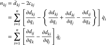
Since the inertia matrix D(q) is symmetric, that is, dij = dji, it follows from Equation (6.113) by interchanging the indices k and j that

which completes the proof.
It is important to note that, in order for  to be skew-symmetric, one must define C according to Equation (6.67). This will be important in later chapters when we discuss robust and adaptive control algorithms.
Related to the skew symmetry property is the so-called passivity property which, in the present context, means that there exists a constant, β ⩾ 0, such that
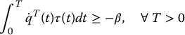
The term  has units of power. Thus, the expression
  is the energy produced by the system over the time interval [0, T]. Passivity means that the amount of energy dissipated by the system has a lower bound given by − β. The word passivity comes from circuit theory where a passive system according to the above definition is one that can be built from passive components (resistors, capacitors, inductors). Likewise a passive mechanical system can be built from masses, springs, and dampers.
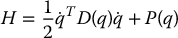
To prove the passivity property, let H be the total energy of the system, that is, the sum of the kinetic and potential energies,
The derivative  satisfies
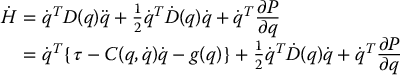
where we have substituted for  using the equations of motion. Collecting terms and using the fact that
  yields
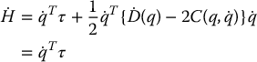
the latter equality following from the skew symmetry property. Integrating both sides of Equation (6.118) with respect to time gives,
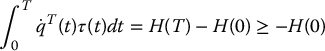
since the total energy H(T) is nonnegative, and the passivity property therefore follows with β = H(0).
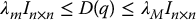
6.5.2 Bounds on the Inertia Matrix
We have remarked previously that the inertia matrix for an n-link rigid robot is symmetric and positive definite. For a fixed value of the generalized coordinate q, let 0 < λ1(q) ⩽ … ⩽ λn(q) denote the n eigenvalues of D(q). These eigenvalues are positive as a consequence of the positive definiteness of D(q). As a result, it can easily be shown that

where In × n denotes the n × n identity matrix. The above inequalities are interpreted in the standard sense of matrix inequalities, namely, if A and B are n × n matrices, then B < A means that the matrix A − B is positive definite and B ⩽ A means that A − B is positive semi-definite.
If all of the joints are revolute, then the inertia matrix contains only terms involving sine and cosine functions and, hence, is bounded as a function of the generalized coordinates. As a result, one can find constants λm and λM that provide uniform (independent of q) bounds in the inertia matrix
6.5.3 Linearity in the Parameters
The robot equations of motion are defined in terms of certain parameters, such as link masses, moments of inertia, etc., that must be determined for each particular robot in order, for example, to simulate the equations or to tune controllers. The complexity of the dynamic equations makes the determination of these parameters a difficult task. Fortunately, the equations of motion are linear in these inertia parameters in the following sense. There exists an n × ℓ function,  and an ℓ-dimensional vector Θ such that the Euler–Lagrange equations can be written as

The function  is called the regressor and
  is the parameter vector. The dimension of the parameter space, that is, the number of parameters needed to write the dynamics in this way, is not unique. In general, a given rigid body is described by ten parameters, namely, the total mass, the six independent entries of the inertia tensor, and the three coordinates of the center of mass. An n-link robot then has a maximum of 10n dynamics parameters. However, since the link motions are constrained and coupled by the joint interconnections, there are actually fewer than 10n independent parameters. Finding a minimal set of parameters that can parameterize the dynamic equations is, however, difficult in general.
Consider the two-link, revolute-joint, planar robot from Section 6.4. If we group the inertia terms appearing in Equation (6.86) as

then we can write the inertia matrix elements as
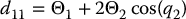


No additional parameters are required in the Christoffel symbols as these are functions of the elements of the inertia matrix. However, the gravitational torques generally require additional parameters. Setting

we can write the gravitational terms g1 and g2 as

Substituting these into the equations of motion it is straightforward to write the dynamics in the form (6.122) where
and the parameter vector Θ is given by
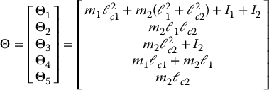
Thus, we have parameterized the dynamics using a five dimensional parameter space. Note that in the absence of gravity only three parameters are needed.
6.6 Newton–Euler Formulation
In this section, we present a method for analyzing the dynamics of robot manipulators known as the Newton–Euler formulation. This method leads to exactly the same final answers as the Lagrangian formulation presented in earlier sections, but the route taken is quite different. In particular, in the Lagrangian formulation we treat the manipulator as a whole and perform the analysis using a Lagrangian function (the difference between the kinetic energy and the potential energy). In contrast, in the Newton–Euler formulation we treat each link of the robot in turn, and write down the equations describing its linear motion and its angular motion. Of course, since each link is coupled to other links, these equations that describe each link contain coupling forces and torques that appear also in the equations that describe neighboring links. By doing a so-called forward-backward recursion, we are able to determine all of these coupling terms and eventually to arrive at a description of the manipulator as a whole. Thus we see that the philosophy of the Newton–Euler formulation is quite different from that of the Lagrangian formulation.
At this stage the reader can justly ask whether there is a need for another formulation. Historically, both formulations were evolved in parallel, and each was perceived as having certain advantages. For instance, it was believed at one time that the Newton–Euler formulation is better suited to recursive computation than the Lagrangian formulation. However, the current situation is that both of the formulations are equivalent in almost all respects. At present the main reason for having another method of analysis at our disposal is that it might provide different insights.
In any mechanical system one can identify a set of generalized coordinates (which we introduced in Section 6.1 and labeled q) and corresponding generalized forces (also introduced in Section 6.1 and labeled τ). Analyzing the dynamics of a system means finding the relationship between q and τ. At this stage we must distinguish between two aspects: First, we might be interested in obtaining closed-form equations that describe the time evolution of the generalized coordinates, such as Equation (6.90). Second, we might be interested in knowing what generalized forces need to be applied in order to realize a particular time evolution of the generalized coordinates. The distinction is that in the latter case we only want to know what time dependent function τ( · ) produces a particular trajectory q( · ) and may not care to know the general functional relationship between the two. It is perhaps fair to say that in the former type of analysis, the Lagrangian formulation is superior while in the latter case the Newton–Euler formulation is superior. Looking ahead to topics beyond the scope of the book, if one wishes to study more advanced mechanical phenomena such as elastic deformations of the links (i.e., if one no longer assumes rigidity of the links), then the Lagrangian formulation is superior.
In this section we present the general equations that describe the Newton–Euler formulation. In the next section we illustrate the method by applying it to the planar elbow manipulator studied in Section 6.4 and show that the resulting equations are the same as Equation (6.90).
The facts of Newtonian mechanics that are pertinent to the present discussion can be stated as follows:
- Every action has an equal and opposite reaction. Thus, if body 1 applies a force f and torque τ to body 2, then body 2 applies a force of − f and torque of − τ to body 1.
- The rate of change of the linear momentum equals the total force applied to the body.
- The rate of change of the angular momentum equals the total torque applied to the body.
Applying the second fact to the linear motion of a body yields the relationship

where m is the mass of the body, v is the velocity of the center of mass with respect to an inertial frame, and f is the sum of external forces applied to the body. Since in robotic applications the mass is constant as a function of time, Equation (6.134) can be simplified to the familiar relationship

where  is the acceleration of the center of mass.
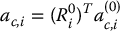
Applying the third fact to the angular motion of a body gives
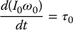
where I0 is the moment of inertia of the body about an inertial frame whose origin is at the center of mass, ω0 is the angular velocity of the body, and τ0 is the sum of torques applied to the body. Now there is an essential difference between linear motion and angular motion. Whereas the mass of a body is constant in most applications, its moment of inertia with respect an inertial frame may or may not be constant. To see this, suppose we attach a frame rigidly to the body, and let I denote the inertia matrix of the body with respect to this frame. Then I remains the same irrespective of whatever motion the body executes. However, the matrix I0 is given by

where R is the rotation matrix that transforms coordinates from the body attached-frame to the inertial frame. Thus there is no reason to expect that I0 is constant as a function of time.
One possible way of overcoming this difficulty is to write the angular motion equation in terms of a frame rigidly attached to the body. This leads to
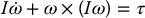
where I is the (constant) inertia matrix of the body with respect to the body-attached frame, ω is the angular velocity, but expressed in the body-attached frame, and τ is the total torque on the body, again expressed in the body-attached frame. Let us now give a derivation of Equation (6.138) to demonstrate clearly where the term ω × (Iω) comes from; note that this term is called the gyroscopic term.
Let R denote the orientation of the frame rigidly attached to the body w.r.t. the inertial frame; note that it could be a function of time. Then Equation (6.137) gives the relation between I and I0. Now by the definition of the angular velocity, we know that
In other words, the angular velocity of the body, expressed in an inertial frame, is given by Equation (6.139). Of course, the same vector, expressed in the body-attached frame, is given by
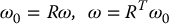
Hence the angular momentum, expressed in the inertial frame, is
Differentiating and noting that I is constant gives an expression for the rate of change of the angular momentum, expressed as a vector in the inertial frame:
Now
Hence, with respect to the inertial frame,
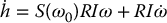
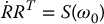
With respect to the frame rigidly attached to the body, the rate of change of the angular momentum is
This establishes Equation (6.138). Of course, if we wish, we can write the same equation in terms of vectors expressed in an inertial frame. But we will see shortly that there is an advantage to writing the force and moment equations with respect to a frame attached to link i, namely that a great many vectors in fact reduce to constant vectors, thus leading to significant simplifications in the equations.
Now we derive the Newton–Euler formulation of the equations of motion of an n-link manipulator. For this purpose, we first choose frames 0, …, n, where frame 0 is an inertial frame, and frame i is rigidly attached to link i for i ⩾ 1. We also introduce several vectors, which are all expressed in frame i. The first set of vectors pertains to the velocities and accelerations of various parts of the manipulator.
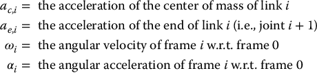
The next several vectors pertain to forces and torques.
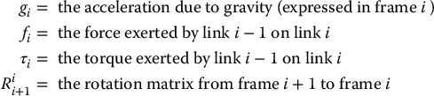
The final set of vectors pertain to physical features of the manipulator. Note that each of the following vectors is constant as a function of q. In other words, each of the vectors listed here is independent of the configuration of the manipulator.
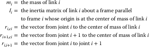
Now consider the free body diagram shown in Figure 6.13; this shows link i together with all forces and torques acting on it. Let us analyze each of the forces and torques shown in the figure. First, fi is the force applied by link i − 1 to link i. Next, by the law of action and reaction, link i + 1 applies a force of − fi + 1 to link i, but this vector is expressed in frame i + 1 according to our convention. In order to express the same vector in frame i, it is necessary to multiply it by the rotation matrix Ri + 1i. Similar explanations apply to the torques τi and − Ri + 1iτi + 1. The force migi is the gravitational force. Since all vectors in Figure 6.13 are expressed in frame i, the gravity vector gi is in general a function of i.

Figure 6.13 Forces and moments on link i
Writing down the force balance equation for link i gives
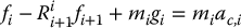
Next we write down the moment balance equation for link i. For this purpose, it is important to note two things: First, the moment exerted by a force f about a point is given by f × r, where r is the radial vector from the point where the force is applied to the point about which we are computing the moment. Second, in the moment equation below, the vector migi does not appear, since it is applied directly at the center of mass. Thus we have
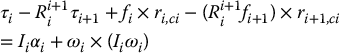
Now we present the heart of the Newton–Euler formulation, which consists of finding the vectors f1, …, fn and τ1, …, τn corresponding to a given set of vectors  . In other words, we find the forces and torques in the manipulator that correspond to a given set of generalized coordinates and first two derivatives. This information can be used to perform either type of analysis, as described above. That is, we can either use the equations below to find the f and τ corresponding to a particular trajectory q( · ), or else to obtain closed-form dynamical equations. The general idea is as follows: Given
  , suppose we are somehow able to determine all of the velocities and accelerations of various parts of the manipulator, that is, all of the quantities ac, i, ωi, and αi. Then we can solve Equations (6.146) and (6.147) recursively to find all the forces and torques, as follows: First, set fn + 1 = 0 and τn + 1 = 0. This expresses the fact that there is no link n + 1. Then we can solve Equation (6.146) to obtain
By successively substituting i = n, n − 1, …, 1 we find all forces. Similarly, we can solve Equation (6.147) to obtain

By successively substituting i = n, n − 1, …, 1 we find all torques. Note that the above iteration is running in the direction of decreasing i.
Thus, the solution is complete once we find an easily computed relation between  and ac, i, ωi, and αi. This can be obtained by a recursive procedure in the direction of increasing i. This procedure is given below, for the case of revolute joints; the corresponding relationships for prismatic joints are actually easier to derive.
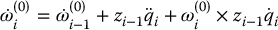
In order to distinguish between quantities expressed with respect to frame i and the base frame, we use a superscript (0) to denote the latter. Thus, for example, ωi denotes the angular velocity of frame i expressed in frame i, while ω(0)i denotes the same quantity expressed in an inertial frame.
Now we have that
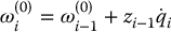
This merely expresses the fact that the angular velocity of frame i equals that of frame i − 1 plus the added rotation from joint i. To get a relation between ωi and ωi − 1, we need only to express the above equation in frame i rather than in the base frame, taking care to account for the fact that ωi and ωi − 1 are expressed in different frames. This leads to
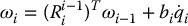
where
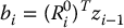
is the axis of rotation of joint i expressed in frame i.
Next let us work on the angular acceleration αi. It is vitally important to note here that
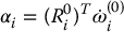
In other words, αi is the derivative of the angular velocity of frame i, expressed in frame i. It is not true that  ! We will encounter a similar situation with the velocity and acceleration of the center of mass. Now we see directly from Equation (6.150) that
Expressing the same equation in frame i gives

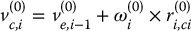
Now we come to the linear velocity and acceleration terms. Note that, in contrast to the angular velocity, the linear velocity does not appear anywhere in the dynamic equations; however, an expression for the linear velocity is needed before we can derive an expression for the linear acceleration. From Section 4.5, we get that the velocity of the center of mass of link i is given by
To obtain an expression for the acceleration, note that the vector r(0)i, ci is constant in frame i. Thus

Now
Let us carry out the multiplication and use the familiar property
We also have to account for the fact that ae, i − 1 is expressed in frame i − 1 and transform it to frame i. This gives

Now to find the acceleration of the end of link i, we can use Equation (6.160) with ri, i + 1 replacing ri, ci. Thus

Now the recursive formulation is complete. We can now state the Newton–Euler formulation as follows.
- Start with the initial conditions
(6.162)and solve Equations (6.151), (6.155), (6.161), and (6.160) (in that order) to compute ωi, αi, and ac, i for i increasing from 1 to n.

- Start with the terminal conditions
(6.163)and use Equations (6.148) and (6.149) to compute fi and τi for i decreasing from n to 1.
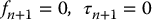
6.6.1 Planar Elbow Manipulator Revisited
In this section we apply the recursive Newton–Euler formulation derived in Section 6.6 to analyze the dynamics of the planar elbow manipulator of Figure 6.9, and show that the Newton–Euler method leads to the same equations as the Lagrangian method, namely Equation (6.90).
We begin with the forward recursion to express the various velocities and accelerations in terms of q1, q2, and their derivatives. Note that, in this simple case, it is quite easy to see that

so that there is no need to use Equations (6.151) and (6.155). Also, the vectors that are independent of the configuration are as follows:


where i here denotes the unit vector (1, 0, 0) and not the index i in the iteration.
Forward Recursion Link 1
Using Equation (6.160) with index i = 1 and noting that ae, 0 = 0 gives
where, again i and j the standard unit vectors in the x and y directions, respectively. Notice how simple this computation is when we do it with respect to frame 1, as opposed to the same computation in frame 0. Finally, we have
where g is the acceleration due to gravity. At this stage we can economize a bit by not displaying the third components of these accelerations, since they are all equal to zero. Similarly, the third component of all forces will be zero while the first two components of all torques will be zero. To complete the computations for link 1, we compute the acceleration of end of link 1. This is obtained from Equation (6.167) by replacing ℓc1 by ℓ1. Thus
Forward Recursion: Link 2
Once again we use Equation (6.160) and substitute for ω2 from Equation (6.164). This yields
The only quantity in the above equation which is configuration dependent is the first one. This can be computed as
Substituting into Equation (6.170) gives
The gravitational vector is
Since there are only two links, there is no need to compute ae, 2. Hence the forward recursions are complete at this point.
Backward Recursion: Link 2
Now we carry out the backward recursion to compute the forces and joint torques. Note that, in this instance, the joint torques are the externally applied quantities, and our ultimate objective is to derive dynamical equations involving the joint torques. First we apply Equation (6.148) with index i = 2 and note that f3 = 0. This results in
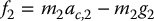

Now we can substitute for ω2, α2 from Equation (6.164), and for ac, 2 from Equation (6.172). We also note that the gyroscopic term equals zero, since both ω2 and I2ω2 are aligned with k. Now the cross product f2 × ℓc2i is clearly aligned with k, the unit vector in the z direction, and its magnitude is just the second component of f2. The final result is

Since τ2 = τ2k, we see that the above equation is the same as the second equation in (6.90).
Backward Recursion: Link 1
To complete the derivation, we apply Equations (6.148) and (6.149) with index i = 1. First, the force equation is
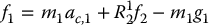
and the torque equation is
Now we can simplify things a bit. First, R12τ2 = τ2, since the rotation matrix does not affect the third components of the vectors. Second, the gyroscopic term is again equal to zero. Finally, when we substitute for f1 from Equation (6.177) into Equation (6.178), a little algebra gives
Once again, all these products are quite straightforward, and the only difficult calculation is that of R12f2. The final result is:
If we now substitute for τ1 from Equation (6.176) and collect terms, we will get the first equation in (6.90); the details are routine and are left to the reader.
6.7 Chapter Summary
In this chapter we treated the dynamics of n-link rigid robots in detail. We derived the Euler–Lagrange equations from D’Alembert’s principle and the principle of virtual work. These equations take the form
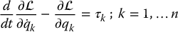
where n is the number of degrees of freedom and  is the Lagrangian function; the difference of the Kinetic and Potential energies, which are written in terms of a set of generalized coordinates (q1, …, qn). The terms τk are generalized forces acting on the system.
We derived computable formulas for the kinetic and potential energies; the kinetic energy  is given as
where
is the n × n inertia matrix of the manipulator. The matrices Ii in the above formula are the link inertia tensors. The inertia tensor is computed in a body-attached frame as

where
and
are the principal moments of inertia and cross products of inertia, respectively, where the integration is taken over the region of space occupied by the body.
The formula for the potential energy of the ith link is
where g is gravity vector expressed in the inertial frame and the vector rci gives the coordinates of the center of mass of link i in the inertial frame. The total potential energy of the n-link robot is therefore
We then derived a special form of the Euler–Lagrange equations using the above expressions for the kinetic and potential energies as
where the terms

are gravitational generalized forces

and the terms cijk are Christoffel symbols of the first kind.
In vector-matrix form the Euler–Lagrange equations become

where the (k, j)th element of the matrix  is defined as
and the gravity vector g(q) is given by
Next, we derived some important properties of the Euler–Lagrange equations, namely, the properties of skew symmetry, passivity, and linearity in the parameters. The skew symmetry property states that the matrix  . The passivity property states that there exists a constant β > 0 such that

The linearity-in-the-parameters-property states that there exists an n × ℓ function,  , called the regressor, and an ℓ-dimensional vector Θ, called the parameter vector such that the Euler–Lagrange equations can be written

We also derived bounds on the inertia matrix for an n-link manipulator as

In case the robot contains only revolute joints, the functions λ1 and λn can be chosen as positive constants.
Finally, we discussed the recursive Newton–Euler formulation of robot dynamics. The Newton–Euler formulation is equivalent to the Euler–Lagrange method but offers some advantages from the standpoint of online computation.
Problems
- Complete the derivation of the dynamic equations for the single-link, flexible-joint robot in Example 6.2.
- Verify Equation (6.21) by direct calculation, neglecting quadratic terms in δr1 and δr2.
- Consider a rigid body undergoing a pure rotation with no external forces acting on it. The kinetic energy is then given as
with respect to a coordinate frame located at the center of mass and whose coordinate axes are principal axes. Take as generalized coordinates the Euler angles ϕ, θ, ψ and show that the Euler–Lagrange equations of motion of the rotating body are

- Find the moments of inertia and cross products of inertia of a uniform rectangular solid of sides a, b, c with respect to a coordinate system with origin at the one corner and axes along the edges of the solid.
- Given the inertia matrix D(q) defined by Equation (6.86) show that
 for all q.
 - Show that the inertia matrix D(q) for an n-link robot is always positive definite.
- Verify the expression (6.62) that was used to derive the Christoffel symbols.
- Consider a 3-link Cartesian manipulator,
- Compute the inertia tensor Ji for each link i = 1, 2, 3 assuming that the links are uniform rectangular solids of length 1, width
 , and height
  , and mass 1.
 - Compute the 3 × 3 inertia matrix D(q) for this manipulator.
- Show that the Christoffel symbols cijk are all zero for this robot. Interpret the meaning of this for the dynamic equations of motion.
- Derive the equations of motion in matrix form:

- Compute the inertia tensor Ji for each link i = 1, 2, 3 assuming that the links are uniform rectangular solids of length 1, width
- Derive the Euler–Lagrange equations for the planar RP robot in Figure 3.14.
- Derive the Euler–Lagrange equations for the planar RPR robot in Figure 5.14.
- Derive the Euler–Lagrange equations of motion for the three-link RRR robot of Figure 5.13. Explore the use of symbolic software, such as Maple or Mathematica, for this problem. See, for example, the Robotica package [126].
-
For each of the robots above, define a parameter vector, Θ, compute the regressor,
 and express the equations of motion as
(6.181)
and express the equations of motion as
(6.181)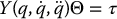
-
Recall for a particle with kinetic energy
 , the momentum is defined as
Therefore, for a mechanical system with generalized coordinates q1, …, qn, we define the generalized momentum pk as

where L is the Lagrangian of the system. With
 and L = K − V prove that

-
There is another formulation of the equations of motion of a mechanical system that is useful, the so-called Hamiltonian formulation. Define the Hamiltonian function H by
- Show that H = K + V.
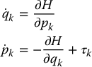
- Using the Euler–Lagrange equations, derive Hamilton’s equations
where τk is the input generalized force.
- For two-link manipulator of Figure 6.9 compute Hamiltonian equations in matrix form. Note that Hamilton’s equations are a system of first-order differential equations as opposed to a second-order system given by Lagrange’s equations.
-
Given the Hamiltonian H for a rigid robot, show that

where τ is the external force applied at the joints. What are the units of
 ?
?
Notes and References
A general reference for dynamics is [55]. More advanced treatments of dynamics can be found in [2] and [112]. The Lagrangian and recursive Newton–Euler formulations of the dynamic equations are given in [64]. These two approaches are shown to be equivalent in [152]. A detailed discussion of holonomic and nonholonomic constraints is found in [85]. The same reference also treats both the Lagrangian and Hamiltonian formulations of dynamics in detail. The properties of skew symmetry and passivity are discussed in [153], [86], and [131]. Parametrization of robot dynamics in terms of a minimal set of inertia parameters is treated in [51]. Identification of manipulator inertia parameters is discussed in [50].